About us

The FAIR standard

• Findability, Accessibility, Interoperability, and Reusability[1].

• Developed by diverse stakeholders (academia, industry, funders, publishers).

• Addressed the need for infrastructure supporting data reuse.

• Emphasis on both human and machine readability.

Why strive for reproducible research?

• Replication crisis: Allows our work to be verified more thoroughly
• Improves science for all: Allows others to more easily build upon our work

Don’t just take our word for it, research funders are increasingly focused on reproducible research too.

Why for reproducible research?

• Open source
• Large active user community for support
• Packages to suit just about every research need: statistics, modelling, spatial analysis, visualisation (Many packages developed by academics)

But just using doesn’t necessarily make your research reproducible…

Workshop concept

Research projects with R

Research projects with R

Graphical overview of components of a good research project in R

1. Rstudio projects

setwd("C:/Users/ben/path/that/only/I/have")

1. Rstudio projects

Stay away from setwd()!

Use Rstudio Projects:

• Designates new or existing folders as working directory creating an .RProj file within them.

• When you open a project the working directory will automatically be set and all paths will be relative to this.

• The .Rproj can be shared along with the rest of the research project, users can easily open the project to have the same working directory.

1. Rstudio projects

Creating projects

Go to File > New Project, can be created in a new or existing directory

1. Rstudio projects

Opening projects

Using File > Open Project in the top left of Rstudio.

1. Rstudio projects

Opening projects

Using the drop down menu in the top-right of the Rstudio session.

1. Rstudio projects

Opening projects

Outside of R by double clicking on the .Rproj file in the folder.

1. Rstudio projects

Utilising project specific .Rprofile’s

• Rstudio projects can store project-specific settings using the .Rprofile file.

• File is run every time the project is opened, can be used to perform actions such as opening a particular script:

setHook("rstudio.sessionInit", function(newSession) {
  if (newSession)
    # Open the script specificed by the path
    rstudioapi::navigateToFile('scripts/script_to_open.R', line = -1L, column = -1L)
}, action = "append")

1. Rstudio projects

Utilising project specific .Rprofile’s

The easiest way to create and edit .Rprofile files is to use the functions from the package usethis:

# Note the use of scope = "project" to create a project specific .Rprofile
usethis::edit_r_profile(scope = "project")

2. Environment management

Familiar lines from the beginning of many an R script:

install.packages("ggplot2")
library(ggplot2)

Again, what is wrong?

2. Environment management

2. Environment management

But the problem is bigger than just packages…

When your code runs it is also utilizing:

• A specific version of R

• A specific operating system

• Specific versions of system dependencies, i.e. other software that R packages utilise.

Collectively, these are the Environment of your code, documenting and managing this is essential ensure reproducibilty

2. Environment management

But how to manage your environment?

• Different approaches that range in complexity hence maybe suited to some projects and not others.

• Most user-friendly way to manage your package environment (caveat to be discussed) in R: renv package.

2. Environment management

Creating reproducible environments with renv

renv helps you create reproducible environments for your R projects by:

• Documenting your package environment

• Providing functionality to re-create it.

2. Environment management

Creating reproducible environments with renv

• Normally all your R packages are stored in a single library on your machine (system library).
• renv creates a project specific libraries of packages (renv/library) which contain all the packages used by your project.
• renv also creates project specific lockfiles (renv.lock) which contain sufficient metadata so that the project library can be re-installed on a new machine.

Result: Different projects can use different versions of packages and installing, updating, or removing packages in one project doesn’t affect any other project.

2. Environment management

renv limitation

renv is not intended to manage other aspects of your environment such as: tracking your version of R or your operating system.

This is why if you want ‘bullet-proof’ reproducibility renv needs to be used alongside other approaches such as containerization.

3. Writing clean code

• There is no objective measure that makes code ‘clean’ vs. ‘un-clean’.

• Think of ‘clean coding’ as the pursuit of making your code easier to read, understand and maintain.

3. Writing clean code

Code styles

• Like writing, code should follow a set of rules and conventions. For example, in English, a sentence starts with a capital letter and ends with a full stop.

• For R code there is not a single set of conventions instead there are numerous styles. Two most common are the Tidyverse style and the Google R style.

Most important: Choose a style and apply it consistently in your coding.

3. Writing clean code

Code styles

Code styles express opinionated preferences on a series of common topics:

• Object naming
• Use of assignment operators
• Spacing
• Indentation
• Line length
• Parentheses placement

We won’t discuss in detail but you should read one of the style guides when you have the time.

3. Writing clean code

Automating the styling of your code

Two R packages for code styling, lintr and styler:

• lintr checks your code for style issues and potential programming errors then presents them to you to correct, like doing a ‘spellcheck’ on a written document.
• styler automatically format’s your code to a particular style, the default of which is the tidyverse style.

3. Writing clean code

Automating the styling of your code

• To use lintr and styler call their functions like any package

• styler can also be used through the Rstudio Addins menu below the Navigation bar:

• Both packages can be used as part of a continuous integration (CI) workflow with Github, meaning that their functions can be run automatically when you update your code.

3. Writing clean code

Script headers

• Starting your scripts with a consistent header containing information about it’s purpose, author/s, creation and modification dates is very helpful!

• There are no rules as to what this should look like but this is an example:

```{r}
#############################################################################
## Script_title: Brief description of script purpose
##
## Notes: More detailed notes about the script and it's purpose
##
## Date created: 
## Author(s):
##################################################################
```

3. Writing clean code

Script headers

3. Writing clean code

Script headers

To use a code snippet simply start typing the keyword in the script and the auto-completion list will appear then press Tab and the code section will be inserted:

3. Writing clean code

Code sections

• Braced ({}) sections of code (i.e. function definitions, conditional blocks, etc.) can be folded to hide their contents by clicking on the small triangle in the left margin:

• But you can also create custom named code sections to break longer scripts according to specific parts of the analysis.

3. Writing clean code

Code sections

• Code sections are created by inserting a comment line that contains at least four trailing dashes (-), equal signs (=), or pound signs (#):

• Alternatively you can use the Code > Insert Section command.

3. Writing clean code

Code sections

To navigate between code sections:

• Use the Jump To menu available at the bottom of the editor[4]

3. Writing clean code

Code sections

To navigate between code sections:

• Use the document outline pane in the top right corner of the source pane

4. Workflow decomposition

• Workflow decomposition is the structuring or compartmentalising of code into seperate logical parts that makes it easier to maintain [5].

• You probably already instinctively do decomposition by splitting typical processes such as:

  • Data preparation
  • Statistical modelling
  • Analysis of results
  • Producing final visualizations

• This oftens leads to scripts with logical sounding names like: Data_prep.R and Data_analysis.R but can others be expected to know which order these must be run in?

4. Workflow decomposition

Solutions:

• 1st step: Give your scripts sequential numeric tags in their names, e.g. 01_Data_prep.R, 02_Data_analysis.R ensuring that they are presented in numerical order in their designated directory.

• Next level: Create a Master script that sources your other scripts in sequence (think of them as sub-scripts) so that users need only run one script.

4. Workflow decomposition

• To do this create the master script as you would any normal R script (File > New File > R script) and then use the base::source() function to run the sub-scripts:

#############################################################################
## Master_script: Run steps of research project in order
#############################################################################

#Prepare LULC data
source("Scripts/Preparation/Dep_var_dat_prep.R", local = scripting_env)

#Prepare predictor data
source("Scripts/Preparation/Ind_var_data_prep.R", local = scripting_env)

• Another advantage of this approach is that all sub-scripts can utilise the same environment (defined by the source(local= ) argument).

4. Workflow decomposition

• Within your sub-scripts processes should also be seperated into code sections and any repetitive tasks should be performed with custom functions.

• Following this approach you end up with a workflow that will look something like this:

5. Structuring your project directory

• A clean project directory that has well-organised sub-directories makes your projects code easier to understand for others.

• Try to use:

  • Logical naming
  • A consistent style (i.e. use of captialisation and seperators).
  • Nested sub-directories e.g data/raw/climatic/precipitation/2020/precip_2020.rds vs. data/precip_2020_raw.rds (helpful when it comes to programatically constructing file paths)

5. Structuring your project directory

As an example my go-to project directory structure looks like this:

└── my_project
    ├── data # The research data
    │   ├── raw
    │   └── processed
    ├── output # Storing results
    ├── publication # Containing the academic manuscript of the project
    ├── src # For all files that perform operations in the project
    │   ├── scripts
    │   └── functions
    └── tools # Auxilliary files and settings

5. Structuring your project directory

• Creation of project directory structure can be automated using using Rstudio’s Project Templates functionality.

• Allows selection of custom template when creating a new Rstudio project (File > New Project > New Directory > New Project Template).

• Warning: Implementation of personal template is labor intensive as it needs to be contained within an R-package. But several template packages appropriate for scientific research projects are available:

  • rrtools
  • ProjectTemplate
  • template
  • addinit

6. Project documentation

Singer 2024

6. Project documentation

But writing comprehensive documentation that covers all aspects of projects is time-consuming…

Suggested solution in the R research community: Research as package approach (i.e. creating your project as an R-package) [6].

Pro: R-packages have an existing strict set of conventions for documentation

Cons:

• Learning curve for those unfamiliar with R-packages

• May not be appropriate for all project requirements.

6. Project documentation

Our advice: don’t let the perfect be the enemy of the good and focus on these key areas:

• Provide adequate in-script commentary: Remember that comments should be used to explain the purpose of the code, not what the code is doing

• Document your functions with roxygen skeletons

• Include a README file: README files are where you should document your project at the macro-level i.e. what it is about and how it is supposed to work.

6. Project documentation

Function documentation with roxygen2

• base R provides a standard way of documenting functions in packages as seperate .Rd (R documentation) files.

• .Rd files use a custom syntax to detail key aspects of the functions such as input parameters, outputs, package dependencies [7].

• Documenting functions in this way is a good practice for your project even if you are not creating a package.

6. Project documentation

Function documentation with roxygen2

• Rather than manually create .Rd files, we can use the roxygen2 package.

• roxygen2 provides functionality to add blocks of comments (roxygen skeleton) to the top of the function scripts. These are then used to automatically generate .Rd files.

• To add a roxygen skeleton, place your cursor inside a function you want to document and press Ctrl + Shift + R (or Cmd + Shift + R on Mac) or you can go to code tools > insert roxygen skeleton (wand icon in the top row of the source pane).

6. Project documentation

Function documentation with `roxygen2

• When you insert the roxygen block it will already contain the names of the function, its arguments and any returns. You can then fill in the rest of the information, such as the description and dependencies etc.

Inserting roxygen block

6. Project documentation

Tips for README writing

• R packages or projects typical have README.md files.
• .md is the Markdown format which is the most common format for README files in R projects because it can be read by many programs and rendered in a variety of formats.
• README.md files are often accompanied by the corresponding file README.Rmd, an Rmarkdown file which generates them.
• README.Rmd files can be created using the usethis package (use_readme_rmd()).
• However, depending on anticipated project users creating the README as a raw text file (.txt) may be better.

6. Project documentation

Tips for README writing

• No single standardised format for what should be included but here is an example of a README.txt file from one of the authors publications.

• Useful to include a tree diagram of the project directory structure down to the file level:

├── Data
│       Raw
│         └── RiceFarms.csv
│        Processed
│         └── RiceFarms_summary.csv
├── Output 
│   └── Regional_size_summary_bar.png 
├── Scripts     
    └── 01_data_analysis.R     
    └──02_data_visualisation.R

6. Project documentation

Tips for README writing

• Such a diagram can be easily generated using the fs package:

install.packages("fs")
library(fs)

#vector path of the target directory to make a file tree from
Target_dir <- "Your_dir"

#produce tree diagram of directory sub-dirs and files and save output using capture.ouput from base R utils.
capture.output(dir_tree(Target_dir), file= 'Dir_tree_output.txt')

Summary

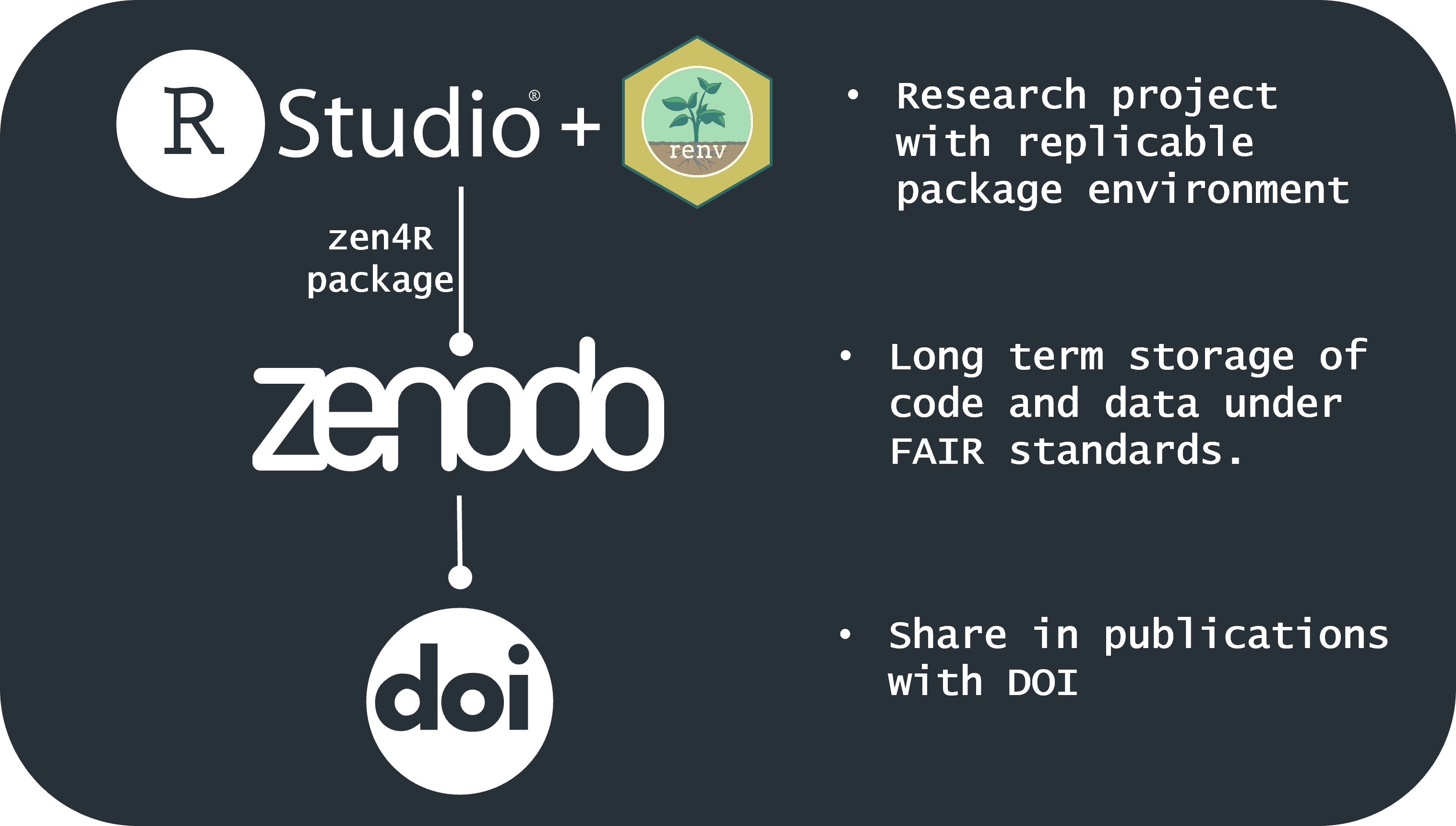
Now this some of the details of the graphical overview probably make more sense to you:

We will implement some of these good practices in our 1st exercise.

Workflows for Reproducibility

We will discuss three workflows for reproducibility:

Rstudio project to Zenodo pipeline

Rstudio project to Zenodo pipeline

Managing Project Environments with renv

• renv creates project-specific libraries

• Captures package versions in a renv.lockfile

• Ensures reproducibility of package environment

• Centralizes package environment management within each project

Rstudio project to Zenodo pipeline

renv Workflow

• Initialize renv inside the project directory to identify dependencies using renv::init()

• Snapshot dependencies to create a lockfile using renv::snapshot()

• Restore environments using renv::restore()

• Easy integration with RStudio for workflow management

Rstudio project to Zenodo pipeline

Limitations of renv

• Does not manage R versions or system-wide dependencies

• Focuses on managing package environments within R

• Best combined with containerization (e.g., Docker) for full reproducibility

• Complements external repositories (e.g., Zenodo) for sharing and preservation

Rstudio project to Zenodo pipeline

Publishing and Archiving with Zenodo

• Long-term storage with generous 50GB upload limit per record

• Permanent DOIs for easy citation and versioning support for updates

• GitHub integration for seamless code archiving with DOI snapshots

• Supports FAIR principles: aligned with open access, transparency, and reusability

• Community creation for grouping related research outputs

• API and open-source: flexible for programmatic access and customization

Rstudio project to Zenodo pipeline

Streamlining publishing to Zenodo with zen4R

• Upload datasets, code, and metadata from R to Zenodo

• Automate publication and deposition management

• Retrieve and update Zenodo records directly in R

• Facilitates integration and reproducibility in R workflows

Rstudio project to Zenodo pipeline

Combining renv and Zenodo

• renv manages internal project environments

• Zenodo ensures external reproducibility with archiving

• Together, they provide a comprehensive solution

• Aligns with open science and FAIR principles

Containerization with Docker

What is containerization?

Containerization is the process of bundling code along with all of it’s dependencies including:

• The operating system

• Software libraries (packages)

• Other system software

Everything needed to run the code is included means that the code is portable and can be run on any platform or cloud service.

This makes containerization the gold standard for reproducibility

Containerization with Docker

What is Docker?

Containerization with Docker

Dockerfile:

• Text file containing a collection of commands to create a new Docker Image.
• Includes the details of the environment required to create to run the code and the command to do it.
• Typically start from a base image, i.e an existing Docker Image.

Containerization with Docker

Docker Image:

• A read-only file that contains the instructions for creating a Docker Container.
• Blueprint of what will be in a container when it is running.
• Docker Images can be shared via Dockerhub, so that they can be used by others.

Containerization with Docker

Docker Container:

• A running instance of a Docker image that runs code with it’s environment
• Runs in isolation from the host, only accesses host files (i.e. data) if it has been configured to do so.
• Possible to create multiple containers simultaneously from the same Docker Image.

Containerization with Docker

Using Docker with R

Two main resources that can help in the creation of containerized R projects:

1. Rocker:

• A project that catalogs and manages Docker Images for R projects.

• Basic images include different versions of R and RStudio

• Other images offering collections of R packages for specific purposes (e.g. tidyverse).

Containerization with Docker

Using Docker with R

Two main resources that can help in the creation of containerized R projects:

2. Dockerfile:

• A package which creates a custom class object that represents the Dockerfile

• Has slots corresponding to common elements of Docker images allowing to add elements to the dockerfile in R.

Containerization with Docker

Docker with renv

Two methods of integrating renv with Docker to manage the package environment of your project:

1. Use renv to install packages when the Docker image is built:

• Useful for multiple projects with identical package requirements because you can re-use the image as a base for new images[8].
• Restoring the package library (renv::restore()) when building the image is slow so try to avoid the need to re-build the base image many times.

Containerization with Docker

Docker with renv

Two methods of integrating renv with Docker to manage the package environment of your project:

2. Use renv to install/restore packages only when Docker containers are run:

• Better when you plan to have multiple projects built from the same base image but with different package requirements.

• Package library is not included in the image but instead different project specific libraries are mounted to the container when it is run [8].

• If renv::restore() is run with caching, packages are not re-installed everytime the container is run.

Version control with Github

Why Git and GitHub?

• Version control: A more systematic way to organise data beyond “dataprep_1”, “dataprep_final”, “dataprep_finalfinal” etc.

• Systematic documentation and storage of code changes allowing us to track changes and revert back to previous versions when needed.

Version control with Github

Terminologies

• Push and Pull?

Git terminologies

• Git cheatsheet: https://education.github.com/git-cheat-sheet-education.pdf

Version control with Github

Steps for using Git and GitHub (To be done in the exercises - basic)

• Create a GitHub repository in your account

• Download and install Git

• Add credentials for your account to Git

• Link RProject to Github repository

• Open, checkout and navigate Git repository local version via Rstudio

• Basic functionalities of Git in Rstudio

Version control with Github

Additional fucntionalities

• GitHub repositories can be archived on Zenodo and thus get a DOI.
• GitHub actions
• GitHub releases can be continuously integrated into DockerHub or GitHub Packages

Quarto

Quarto

• Quarto website presents many examples of it’s applications
• We will focus on some of it’s key uses and features that are relevant for academics and producing reproducible research.
  • Academic manuscripts
  • Presentations
  • Websites
  • Interactive dashboards
  • Data exploration and visualization

Quarto

Writing academic manuscripts

How many programs do you currently use when writing academic papers?

A common workflow of academic papers [9]

Quarto

Writing academic manuscripts

Quarto solves this problem by allowing you to write full academic manuscripts from start to finish including text, code, and visualizations in a single document:

Quarto

Writing academic manuscripts

Key benefits:

• Figures and tables are dynamically updated as your code changes
• Supports code in R, Python and Julia as well as LaTeX and Markdown content
• Easy Cross-referencing capability for figures, tables, and sections
• Documents can be rendered as Word, PDF, or HTML
• Include Citations and bibliographies using Crossref, DataCite, PubMed and direct integration with Zotero
• Quarto’s .qmd files can be edited with various code/text editors (VS Code, RStudio etc.)

Quarto

Presentations

Several formats: RevealJS, Microsoft Powerpoint and Beamer using a common syntax.

Useful features:

• Modern themes with functionality to publish your own theme.

• Interactive content: Executable code blocks, graphs, maps

• Dynamic resizing of content depending on screen size

• Functionality for slide notes, automatic transitions, timers etc.

• Easy export to PDF or HTML

• Similar to manuscripts code-based content is dynamically updated.

Quarto

Websites

Websites to act as guides, tutorials or teaching materials:

Quarto

Websites

Personal websites to share publications and presentations:

Quarto

Websites

Websites for research projects to share progress and results:

Quarto

Dashboards

Quarto

Data exploration and visualization

Guided exercises

On the website for the masterclass under the heading Guided exercises you will find 4 exercises that put into practice the workflows we have discussed as well as the starting to write an academic manuscript with Quarto.

• The exercises build incrementally on each other but they don’t need to be completed in order.

• Choose which one interests you most or depending on your existing knowledge and expertise.

• We have allocated 45 minutes to work on the exercises and we will be here to help you if you have any questions.

Discussion and Feedback

This is an open discussion so feel free to raise any points you might have, but here are some ideas:

• Any questions of understanding or clarification about the content we have covered today?

• What are your own experiences with trying to make your work reproducible? Particular successes or obstacles you have encountered?

• Are there any other tools or workflows that you have found useful that you would like to share with the group?

• Have you encountered any particular differences in the way that reproducibility is approached in your field/discipline?

Bibliography

1.
Wilkinson MD, Dumontier M, Aalbersberg IjJ, et al (2016) The FAIRGuidingPrinciples for scientific data management and stewardship. Scientific Data 3(1):160018. https://doi.org/10.1038/sdata.2016.18
Marwick B, Boettiger C, Mullen L (2018) Packaging data analytical work reproducibly using r (and friends). The American Statistician 72(1):80–88. https://doi.org/10.1080/00031305.2017.1375986
and
and  : Workflows for data, projects and publications