This image highlights some the key concepts we will discuss in the workshop, which have been divided into seperate sections:
Background: Some introductory information on why reproducible and transparent research is important.
Research projects with R: Starting from the basics to develop good practice for creating research projects with R, focusing on some features of Rstudio as an Integrated Development Environment that can help ensure your work is reproducible.
Workflows for reproducibility: Here we present three workflows of differing levels of complexity and discusses how they can be combined and which might be best given the research needs.
Quarto: Here we introduce the open-source scientific and technical publishing system Quarto which can be used for numerous academic activities including preparing manuscripts.
Guided Exercises: Now it’s time to get hands-on with some guided exercises to put into practice some of the concepts we have discussed.
1 Background
About us
We are four researchers from the research group Planning of Landscape and Urban Systems (PLUS) at ETH Zürich. Click on the social icons below our pictures to find out more about our individual research or get in touch with us.
Ben Black
Doctoral Researcher
Nivedita Harisena
Doctoral Researcher
Manuel Kurmann
Research Assistant
Maarten Van Strien
Senior scientist
What is reproducible research?
Reproducibility is a key aspect of reliable scientific research. It enables other researchers to reproduce the same results using the original data, code, and documentation [1]. Below are the core principles to ensure reproducibility in research:
1.
Essawy BT, Goodall JL, Voce D, et al (2020) A taxonomy for reproducible and replicable research in environmental modelling. Environmental Modelling & Software 134:104753. https://doi.org/10.1016/j.envsoft.2020.104753
Starts with planning
Reproducibility begins during the planning stage. It is essential to organize data management and ensure clear protocols are in place even before starting the analysis. Consistent Data Storage Regular backups of data are crucial. Storing data in multiple locations ensures accessibility and minimizes the risk of data loss. [2]
Contains clear documentation
Thorough documentation is essential to guarantee that data and methods can be accurately interpreted and reproduced by others. This entails the use of well-organised files and the inclusion of metadata that describes the data, how it was obtained, and how it was processed. [[2]][3]
Utilizes version control
Using version control systems helps track changes in the project over time. This approach preserves the history of the project and facilitates the reversion of files to a previous state in the event of an error. [2]
Is accessible
Data should be stored in nonproprietary, portable formats to ensure broad accessibility and long-term usability. This practice ensures that researchers can access the data without relying on specific software tools. Making data and code publicly available in accessible repositories supports scientific transparency and allows broader use of research outputs. [[2]][3]
By following these steps, researchers contribute to the wider scientific community, ensuring that their work can be efficiently and accurately reproduced by others.
Introducing the FAIR Principles
While the principles above lay the groundwork for reproducibility, the FAIR principles (Findability, Accessibility, Interoperability, and Reusability) provide a more comprehensive framework for enhancing the value of research data in the digital age. These principles expand on reproducibility by emphasizing not only human access to research outputs but also machine actionability, ensuring that data can be effectively found, accessed, and reused by both people and computational tools. [4]
How FAIR Principles Build on Reproducibility
The FAIR principles naturally complement and expand on the core aspects of reproducible research:
Findability reinforces the importance of clear documentation. Assigning persistent identifiers and providing rich metadata makes it easier for researchers and search tools to locate and understand datasets, ensuring that your research remains accessible over time.
Accessibility builds on the concept of using nonproprietary formats. FAIR emphasizes that data should be retrievable using open, standardized protocols, which ensures long-term access to both the data and its metadata, even if the data itself becomes unavailable.
Interoperability relates to the consistent use of data standards and version control. By using standardized formats and vocabularies, research data can be more easily integrated with other datasets, supporting reuse and long-term relevance in broader research contexts.
Reusability directly aligns with the goals of reproducible research by ensuring that data is accompanied by clear licensing and provenance, allowing others to confidently reuse it. This principle reinforces the need for thorough documentation and transparent methods.
By incorporating the FAIR principles, researchers ensure that their data not only meets the standards of reproducibility but is also optimized for long-term use and discovery. This fosters a research environment where data is more transparent, accessible, and impactful over time. [4]
Why strive for reproducible research?
In recent years, various scientific disciplines have experienced what is known as a “replication crisis”. This crisis arises when researchers are unable to reproduce the headline results of key studies using the reported data and methods [[5]][6][7]. This lack of reproducibility undermines public trust in science, as it raises doubts about the validity of research findings.
5.
Moonesinghe R, Khoury MJ, Janssens ACJW (2007) Most PublishedResearchFindingsAreFalse—But a LittleReplicationGoes a LongWay. PLOS Medicine 4(2):1–4. https://doi.org/10.1371/journal.pmed.0040028
Conducting reproducible research simplifies the process of remembering how and why specific analyses were performed. This makes it easier to explain your work to collaborators, supervisors, and reviewers, enhancing communication throughout your project. [2]
Efficient
Modifications Reproducible research enables you to quickly adjust analyses and figures when requested by supervisors, collaborators, or reviewers. This streamlined process can save substantial time during revisions. [2]
Streamlined Future Projects
By maintaining well-organized and reproducible systems, you can reuse code and organizational structures for future projects. This reduces the time and effort required for similar tasks in subsequent research. [2]
Demonstrates Rigor and Transparency
Reproducibility demonstrates scientific rigor and transparency. It allows others to verify your methods and results, improving the peer review process and reducing the risk of errors or accusations of misconduct. [2]
Increases Impact and Citations
Making your research reproducible can lead to higher citation rates [8][9]. By sharing your code and data, you enable others to reuse your work, broadening its impact and increasing its relevance in the scientific community. [10][11].
McKiernan EC, Bourne PE, Brown CT, et al (2016) How open science helps researchers succeed. eLife 5:e16800. https://doi.org/10.7554/eLife.16800
10.
Whitlock MC (2011) Data archiving in ecology and evolution: Best practices. Trends in Ecology & Evolution 26(2):61–65. https://doi.org/https://doi.org/10.1016/j.tree.2010.11.006
11.
Culina A, Crowther TW, Ramakers JJC, Gienapp P, Visser ME (2018) How to do meta-analysis of open datasets. Nature Ecology & Evolution 2(7):1053–1056. https://doi.org/10.1038/s41559-018-0579-2
Advantages of Reproducibility for Other Researchers
Facilitates Learning
Sharing data and code helps others learn from your work more easily. New researchers can use your data and code as a reference, speeding up their learning curve and improving the quality of their analyses. [2]
Enables Reproducibility
Reproducible research makes it simpler for others to reproduce and build upon your work, fostering more compatible and robust research across studies. [2]
Error Detection
By allowing others to access and review your data and code, reproducibility helps detect and correct errors, ensuring that mistakes are caught early and reducing the chance of their propagation in future research. [2]
2.
Alston JM, Rick JA (2021) A Beginner’s Guide to ConductingReproducibleResearch. The Bulletin of the Ecological Society of America 102(2):e01801. https://doi.org/10.1002/bes2.1801
Why for reproducible research?
R is increasingly recognized as a powerful tool for ensuring reproducibility in scientific research. Here are some key advantages of using R for reproducible research:
Open Source
Accessibility R is freely available to everyone, eliminating cost barriers and promoting inclusive access to research tools. This open-source model ensures that researchers around the world can use and contribute to its development, fostering a collaborative research environment. [3]
Comprehensive Documentation
R encourages thorough documentation of the entire research process. This ensures that analyses are well-tracked and can be easily replicated across different projects, enhancing the overall transparency and reliability of the research.
Integrated Version Control
R seamlessly integrates with version control systems like Git, allowing researchers to track changes to code, data, and documents. This helps maintain a detailed record of a project’s evolution and ensures that all steps are easily reproducible. [3]
3.
Siraji MA, Rahman M (2023) Primer on ReproducibleResearch in R: EnhancingTransparency and ScientificRigor. Clocks & sleep 6(1):1–10. https://doi.org/10.3390/clockssleep6010001
Consistency Across Platforms
R provides a stable environment that works consistently across different operating systems, whether you are using Windows, Mac, or Linux. This cross-platform consistency greatly enhances the reproducibility of research across diverse systems.
Broad Community Support
The R community is large and active, continuously contributing to the improvement of the software. This broad support makes R a reliable choice for long-term research projects, ensuring that new tools and methods are constantly being developed and shared.
Flexibility and Adaptability
R offers a wide range of tools and functions that can be adapted to various research needs. This flexibility allows researchers to handle diverse tasks within a reproducible framework, making it a versatile tool for projects of all kinds.
2 Research projects with R
Let’s start with a definition of what makes a good R project from Jenny Bryan:
A good R project… “creates everything it needs, in its own workspace or folder, and it touches nothing it did not create.”[12]
This is a good definition that contains concepts, such as the notion that projects should be ‘self-contained’. However we add one more caveat to this definition which is that a good R project should explain itself.
For the purpose of this workshop we will approach this topic by splitting it up into 6 topics which are highlighted in this graphic:
Graphical overview of components of a good research project in R
As you move through these you will see that there are areas of overlap and complementarity between them. These topics are also central to the choice of approaches in the three workflows for reproducibility that we will share.
projects
How many times have you opened an R script and been greeted by this line:
setwd("C:/Users/ben/path/that/only/I/have")
While it is well-intentioned (i.e. avoiding the need to have full paths for all objects that will subsequently be loaded or daved ) the problem with it is obvious: This specific path is only relevant for the author and not other potential users and even for the author it will be invalid if they happen to change computers. The good news is there is a very simple way to avoid having to use setwd() at all by using Rstudio Projects.
Rstudio projects designate new or existing folders as a defined working directory by creating an .RProj file within them. This means that when you open a project the working directory of the Rstudio session will automatically be set to the directory that the .RProj file is located in and the paths of all files in this folder will be relative to this.
The .Rproj file can be shared along with the rest of the research project files meaning that others users can easily open the Project to have the same working directory removing the need for those troublesome setwd() lines.
Creating and opening projects
Creating an Rstudio project is as simple as using File > New Project in the top left and then choosing between creating the Project in a new or existing directory.
There are several ways to open a Project:
Using File > Open Project in the top left of Rstudio.
Using the drop down menu in the top-right of the Rstudio session.
Outside of R by double clicking on the .Rproj file in the folder.
Utilising project specific .Rprofile’s
Another useful feature of Rstudio projects is the ability to store project-specific settings using the .Rprofile file which controls the initialisation behaviour of the R session when the project is opened. A useful application of this for reproducible research projects is automatically open a particular script, for example a master script that runs all the code in the project (which is a concept that will discussed under workflow decomposition).
To do this the contents of your .Rprofile file would like this:
setHook("rstudio.sessionInit", function(newSession) {if (newSession)# Open the script specificed by the path rstudioapi::navigateToFile('scripts/script_to_open.R', line =-1L, column =-1L)}, action ="append")
The easiest way to create and edit .Rprofile files is to use the functions from the package usethis:
# Note the use of scope = "project" to create a project specific .Rprofileusethis::edit_r_profile(scope ="project")
Environment management
These lines of code are also probably familiar from the beginning of many an R script:
install.packages("ggplot2")library(ggplot2)
But what is wrong with these lines?
Well firstly, there is no indication of what version of the package is to be installed and hence if the code installing this package is old it may not work with the most recent version of the package (This is less of a problem for well established packages like the Tidyverse but for less common packages, that may see large changes between versions, it could be substantial).
Secondly, having the user install an unspecified version of a package could also cause dependency conflicts with other packages required by the code. This is because almost all packages have some form of dependency (i.e. they use the functionality of) on other packages. This is shown aptly by the image below which, while out-dated now, showed that in 2014 to install the 7 most popular R packages at the time would actually install 63 packages in total when considering their dependencies.
However the problem is bigger than just packages because when your code runs it is also utilising:
A specific version of R
A specific operating system
Specific versions of system dependencies, i.e. other software in other languages that R packages themselves utilise e.g GDAL for spatial analysis packages like terra.
All of these things together make up what is known as the ‘environment’ of your code. Hence the process of documenting and managing this environment to is ensure that your code is reproducible (i.e. it not only runs but also consistently produces the same results).
There are different approaches to environment management that differ in their complexity and hence maybe suited to some projects and not others. For the purpose of this workshop we will focus on what we have found is one of the most user-friendly ways to manage your package environment (caveat that will be discussed) in R which is the package renv. Below we will introduce this package in more detail as it will form a central part of the three workflows for reproducibility that we present.
Creating reproducible environments with renv
As mentioned above renv is an R package that helps you create reproducible environments for your R projects by not only documenting your package environment but also providing functionality to re-create it.
It does this by creating project specific libraries (i.e. directories: renv/library) which contain all the packages used by your project. This is different from the default approach to package usage and installation whereby all packages are stored in a single library on your machine (system library). Having separate project libraries means “that different projects can use different versions of packages and installing, updating, or removing packages in one project doesn’t affect any other project.” [14]. In order to make sure that your project uses the project library everytime it is opened renv utilises the functionality of .Rprofile's to set the project library as the default library.
Another key process of renv is to create project specific lockfiles (renv.lock) which contain sufficient metadata about each package in the project library so that it can be re-installed on a new machine.
As alluded to, renv does a great job of managing your packages but is not intended to manage other aspects of your environment such as: tracking your version of R or your operating system. This is why if you want ‘bullet-proof’ reproducibility renv needs to be used alongside other approaches such as containerization which is the 3rd and most complex workflow we will discuss.
Writing clean code
The notion of writing ‘clean’ code can be daunting, especially for those new to programming. However, the most important thing to bear in mind is that there is no objective measure that makes code ‘clean’ vs. ‘un-clean’, rather we should of think ‘clean’ coding as the pursuit of making your code easier to read, understand and maintain. Also while we should aspire to writing clean code, it is arguably more important that it functions correctly and efficiently.
The central concept of clean coding is that, like normal writing, we should follow a set of rules and conventions. For example, in English a sentence should start with a capital letter and end with a full stop. Unfortunately, in terms of writing R code there is not a single set of conventions that everyone proscribes to, instead there are numerous styles that have been outlined and the important thing is to choose a style and apply it consistently in your coding.
Perhaps the two most common styles are the Tidyverse style and the Google R style (Which is actually a derivative of the former). Neither style can be said to be the more correct, rather they express opinionated preferences on a series of common topics such as: Object naming, use of assignment operators, spacing, indentation, line length, parentheses placement, etc.
Rather than detail all of these topics here we will focus on just on some related tips that we think are most relevant for scientific research coding, including how to automate the formatting of your code to a particular style. However, we encourage you to go through the different style guides when you have the time.
Script headers
Starting your scripts with a consistent header containing information about it’s purpose, author/s, creation and modification dates is a great step making your workflow more understandable and hopefully reproducible. There are no rules as to what such a header should look like but this is the style I like to use:
############################################################################### Script_title: Brief description of script purpose#### Notes: More detailed notes about the script and it's purpose#### Date created: ## Author(s):#############################################################################
To save time inserting this header into new scripts you use Rstudio’s Code snippets feature. Code snippets are simply text macros that quickly insert a section of code using a short keyword.
To create your own Code snippet go to Tools > Global Options > Code > Edit Snippets and then add a new snippet with your code below it:
To use a code snippet simply start typing the keyword in the script and the auto-completion list will appear then press Tab and the code section will be inserted:
Code sections
As you may already know braced ({}) sections of code (i.e. function definitions, conditional blocks, etc.) can be folded to hide their contents in RStudio by clicking on the small triangle in the left margin.
However, an often overlooked feature is the ability to create named code sections that can be also folded, as well as easily navigated between. These can be used to break longer scripts into a set of discrete regions according to specific parts of the analysis (discussed in more detail later). In this regard, another good tip is to give the resulting sections sequential alphabetical or numerical Pre-fixes. Code sections are created by inserting a comment line that contains at least four trailing dashes (-), equal signs (=), or pound signs (#):
# Section One ---------------------------------# Section Two =================================# Section Three #############################
Alternatively you can use the Code > Insert Section command.
To navigate between code sections:
Use the Jump To menu available at the bottom of the editor[15]
Use the document outline pane in the top right corner of the source pane
Automating the styling of your code
There are two R packages that are very helpful in terms of ensuring your code confirms to a consistent style: lintr and styler.
lintr checks your code for common style issues and potential programming errors then presents them to you to correct, think of it like doing a ‘spellcheck’ on a written document.
styler is more active in the sense that it automatically format’s your code to a particular style, the default of which is the tidyverse style.
To use lintr and styler you call their functions like any package but styler can also be used through the Rstudio Addins menu below the Navigation bar as shown in this gif:
Another very useful feature of both packages is that they can be used as part of a continuous integration (CI) workflow using a version control application like Git. This is a topic that we will cover as part of our Version control with Git workflow but what it means is that the styler and lintr functions are run automatically when you push your code to a remote repository.
Workflow decomposition
In computer sciences workflow decomposition refers to the structuring or compartmentalising of your code into seperate logical parts that makes it easier to maintain [16].
In terms of coding scientific research projects many of us probably already instinctively do decomposition to some degree by splitting typical processes such as data preparation, statistical modelling, analysis of results and producing final visualizations.
However this is not always realized in the most understandable way, for example we may have seperate scripts with logical sounding names like: Data_prep.R and Data_analysis.R but can others really be expected to know exactly which order these must be run in, or indeed whether they even need to be run sequentially at all?
A good 1st step to remedying this is to give your scripts sequential numeric tags in their names, e.g. 01_Data_prep.R, 02_Data_analysis.R. This will also ensure that they are presented in numerical order when placed in a designated directory Structuring your project directory and can be explicitly described in your project documentation.
But you can take this to the next level by creating a Master script that sources your other scripts in sequence (think of them as sub-scripts) so that users of your code need only run one script. To do this is as simple as creating the master script as you would any normal R script (File > New File > R script) and then using the base::source() function to run the sub-scripts:
############################################################################### Master_script: Run steps of research project in order#### Date created: 30/7/2024## Author(s): Jane Doe################################################################################ =========================================================================### A- Prepare dependent variable data### =========================================================================#Prepare LULC datasource("Scripts/Preparation/Dep_var_dat_prep.R", local = scripting_env)### =========================================================================### B- Prepare independent variable data### =========================================================================#Prepare predictor datasource("Scripts/Preparation/Ind_var_data_prep.R", local = scripting_env)### =========================================================================### C- Perform statisical modelling### =========================================================================source("Scripts/Modelling/Fit_stat_models.R", local = scripting_env)
As you can see in this example code I have also made use of a script header and code sections, that were previously discussed, to make the division of sub-processes even clearer. Another advantage of this approach is that all sub-scripts can utilise the same environment (defined by the source(local= ) argument) which means that each individual script does not need to load packages or paths as objects.
Finally, within your sub-scripts processes should also be seperated into code sections and ideally any repetitive tasks should be performed with custom functions which again are contained within their own files.
Following this approach you end up with a workflow that will look something like this:
The benefit of this hierarchical approach to structuring is that it is not only easier to debug and maintain individual processes but it is also more amenable to adding new processes.
Structuring your project directory
Similar to having clean code, having a clean project directory that has well-organised sub-directories goes a long way towards making your projects code easier to understand for others. For software development there are numerous sets of conventions for directories structures although these are not always so applicable for scientific research projects. However we can borrow some basic principles, try to use: - Use logical naming - Stick to a consistent style, i.e. use of captialisation and seperators - Make use of nested sub-directories e.g data/raw/climatic/precipitation/2020/precip_2020.rds vs. data/precip_2020_raw.rds. This is very helpful when it comes to programatically constructing file paths especially in projects with a lot of data.
As an example my go-to project directory structure looks like this:
└── my_project
    ├── data # The research data
    │   ├── raw
    │   └── processed
    ├── output # Storing results
    ├── publication # Containing the academic manuscript of the project
    ├── src # For all files that perform operations in the project
    │   ├── scripts
    │   └── functions
    └── tools # Auxilliary files and settings
Rather than manually create this directory structure everytime you start a new project, save yourself some time and automate it by using Rstudio’s Project Templates functionality. This allows you to select a custom template as an option when creating a new Rstudio project through the New project wizard (File > New Project > New Directory > New Project Template).
To implement this even as an intermediate R user is fairly labor intensive as your custom project directory template needs to be contained within an R-package, in order to be available in the wizard. However, quite a few templates with directory structures appropriate for scientific research projects have been created by others:
addinit (Not a template but an interactive shiny add-in for project creation)
Project documentation
As an example of why documentation is important think about if you bought a new table from Ikea only to excitedly rip open the box and find that there are no instructions for how to assemble it. Sure, you know what a table is supposedly to look like and given enough time you will end up with something that will probably be mostly right but maybe it’s missing small details. Also it will probably take you just as long to take it apart in 5 years time. Well, working with undocumented code for research projects is similar except a lot more complicated!
Writing comprehensive documentation that covers all aspects of our projects is time-consuming which is why it is often neglected. For example, there are a lot of different metadata conventions that exist that you could apply. However, learning and adhering strictly to these can be overwhelming and possibly lead to the opposite effect i.e. they are not simple for others to understand either.
In response to this there has been a movement in the R research community to adopt the research as package approach, which, as the name suggests, involves creating your project as an R-package which has a strict set of conventions for documentation [17]. This is a viable approach for those who are familiar with R-packages but is arguably not the best for all projects and users.
17.
Marwick B, Boettiger C, Mullen L (2018) Packaging data analytical work reproducibly using r (and friends). The American Statistician 72(1):80–88. https://doi.org/10.1080/00031305.2017.1375986
Instead, we would suggest to follow the maxim of not letting the perfect be the enemy of the good and to focus on these key areas:
Provide adequate in-script commentary: This is perhaps contentious for those from a software development community, but given the choice I would rather have to read through a script with too many comments than one with too few. However remember that comments should be used to explain the purpose of the code, not what the code is doing. In line with this use script headers.
Document your functions with roxygen skeletons:
Include a README file: README files are where you should document your project at the macro-level i.e. what it is about and how it is supposed to work.
The latter of these two are more detailed so we have provided further information and tips in sections below.
Function documentation with roxygen2
Base R provides a standard way of documenting a package where each function is documented in an .Rd file (R documentation). This documentation uses a custom syntax to detail key aspects of the functions such as their input parameters, outputs and any package dependencies [18].
In the case of many research projects you will not be creating a package however it is still useful to apply this documentation style to your functions as it is a good way to make them understandable and easier to modify by others. For example, having clear information about the object (e.g. a vector or data.frame) that a function accepts, saves others time in guessing what the function is expecting if they are trying to use new data.
However, rather than manually writing .Rd files, we can use the roxygen2 package to automatically generate these files from a block of comments that are added to the top of the function scripts. To add this comment block, place your cursor inside a function you want to document and press Ctrl + Shift + R (or Cmd + Shift + R on Mac) or you can go to code tools > insert roxygen skeleton (code tools is represented by the wand icon in the top row of the source pane). As you can see in this gif below, when you insert the roxygen block it will already contain the names of the function, its arguments and any returns. You can then fill in the rest of the information, such as the description and dependencies etc. for a guide to these other fields see the roxygen2 documentation.
Inserting roxygen block
Tips for README writing
If you look at the source code of R packages or projects that use R in Github repositories you will see that they all contain README.md files. .md is Markdown format which is the most common format for README files in R projects because it can be read by many programs and rendered in a variety of formats. These files are often accompanied by the corresponding file README.Rmd which generates the README.md file. In this sense writing the README for your project in markdown makes sense and there tools available to help you do this such as the usethis package which has a function use_readme_rmd() that will create a README.Rmd file for you. However, depending on who you anticipate using your project you may also want to create your README as a raw text file (.txt) which may be a more familiar format for some users and again can be opened by many different programs.
Again there is not a single standardised format for what should be included in your README file but here is an example of a README file that was written for one of the authors code/data upload alongside a publication: README.txt
You will see that one of the things this README includes is a tree diagram which shows the directory structure of the project right down to the file level. This is a useful way to give an overview of what users should find included in the project and then explanatory notes can be added to explain the purpose of each file or directory. Such a diagram can be easily generated using the fs package:
install.packages("fs")library(fs)#vector path of the target directory to make a file tree fromTarget_dir <-"YOUR DIR"#produce tree diagram of directory sub-dirs and files and save output using capture.ouput from base R utils.capture.output(dir_tree(Target_dir), file='Dir_tree_output.txt')
3 Workflows for Reproducibility
For this workshop we will outline three different workflows for creating reproducible research projects with R combined with other tools. We have named these workflows as follows:
to pipeline
Containerization with
Version control with
These workflows are inter-related in the sense that 2. and 3. build upon elements of the first and indeed the techniques of the latter workflows can also be combined together. The workflows differ in the level of reproducibility they ensure but the trade-off for better reproducibility is increased complexity. As such we would suggest that the most reproducible workflow may not always be the most appropriate to implement dependent on the needs of your research project and the capabilities of the collaborators involved.
Of course, these workflows are by no-means the only way of doing things and indeed we would actively encourage you to expand upon them in developing your own preferred approach.
project to pipeline
The graphic above shows the main steps of this workflow. It starts by developing your research project as an Rstudio project following the good practice project guidelines we have discussed. Then, it uses the renv package to manage the project environment so that others can re-create it. Finally, the code, data and environment are uploaded to the open-access repository Zenodo, which provides a DOI for your work, ensuring long-term accessibility and reproducibility.
The renv package helps maintain the R environment, allowing others to recreate the environment in which your analysis was conducted. By combining renv with Zenodo, you create a comprehensive solution for reproducible research. renv ensures that the computational environment is captured, while Zenodo makes your research outputs accessible and citable, supporting the FAIR principles of findability, accessibility, interoperability, and reusability [4].
4.
Wilkinson MD, Dumontier M, Aalbersberg IjJ, et al (2016) The FAIRGuidingPrinciples for scientific data management and stewardship. Scientific Data 3(1):160018. https://doi.org/10.1038/sdata.2016.18
renv is a powerful R package designed to help manage project environments by creating project-specific libraries and lockfiles. As mentioned earlier, renv captures the exact versions of R packages used in a project, storing this information in a renv.lock file. This allows users to recreate the exact package environment when revisiting a project or transferring it to a different machine, ensuring reproducibility.
The renv workflow is straightforward:
Initialize renv in a project: renv creates a separate library in the project folder, isolating the packages from the system-wide library.
Snapshot dependencies: renv scans the project, identifying which packages are being used and recording their versions in the lockfile.
Restore environments: Anyone cloning or receiving the project can run renv::restore() to install the exact versions of the packages listed in the lockfile from the project library, reproducing the original project package environment.
One of the core strengths of renv is its flexibility. It integrates seamlessly with tools like RStudio, allowing easy management of dependencies without disrupting existing workflows. This makes it particularly well-suited for ensuring that research projects are reproducible across different systems and platforms.
However, renv does not manage the entire system environment (such as the version of R itself or external dependencies like system libraries). For complete reproducibility, combining renv with
containerization tools (like Docker) or publishing outputs (such as code or data) via repositories like Zenodo is recommended.
as a research repository
Zenodo is a platform created under the European Commission‘s OpenAIRE project in partnership with CERN to publish, archive, and share scientific research outputs, including datasets, code, and publications.
Of course there are many other similar research repositories, such as Dryad, Figshare, Mendeley Data and OSF, but we recommend Zenodo for several reasons:
Generous upload size of 50GB (100 files) per record
Aligns with FAIR and Open Science principles: The practical features of Zenodo that ensure this are described in it‘s principles
Ability to create communities: Zenodo Communities are used to group similar records together. This is useful for creating a collection of related research outputs, either for a research group or a large-scale funded project.
Long term preservation with assignment of DOIs: Each item published on Zenodo is assigned a permanent Digital Object Identifier (DOI), which is a better way than a URL to cite the record in academic writing.
Open source: This means that Zenodo is not just free to use but you can even see the code it is built on and contribute to it.
Versioning functionality: Every record starts with a 1st version and new versions can be added as research is updated, while earlier versions remain accessible. This is crucial in scientific research, where updated analyses and data corrections are often necessary, but also transparency around earlier versions of the work should be maintained.
Integration with GitHub: When a research project (e.g., code) is hosted on GitHub, Zenodo can be used to archive the repository upon each new release, creating a snapshot with a DOI. This means that a version of the code can be more easily cited in scientific publications.
Application programming Interface (API) to access records programmatically: This a useful feature as it allows for interfacing with Zenodo records without using the website and is the backbone of the zen4R package that allows for publishing records directly from R which we discuss in more detail below.
Publishing to Zenodo with zen4R
The zen4R package [19] provides functions to interact with Zenodo‘s API directly from R. The package allows you to:
Retrieve the metadata of, and download, existing Zenodo records.
Create new records and versions of records, write their metadata and upload files to Zenodo.
We will use zen4R to publish the code, data, and environment of our example project to Zenodo in the accompanying exercise.
Containerization with
The title of this workflow raises two questions, the first being: what is containerization? and the second: what is Docker? ### Containerisation
Simply put containerization is the process of bundling code along with all of it’s dependencies, i.e. all the components we discussed as making up the environment, including the operating system, software libraries (packages), and other system software. The fact everything needed to run the code is included means that the code is portable and can be run on any platform or cloud service. This also makes containerization something of a gold standard for reproducibility as the entire environment is explicitly re-produced.
Docker
Docker is an open-source, and the most popular, platform for containerization. Before we dive into a practical example using Docker for research projects with R it is important to introduce some three key terms that we will come across:
Dockerfile: The first step in the containerization process, they are a straightforward text file containing a collection of commands or procedures to create a new Docker Image. In this sense we can consider a Dockerfile are the source code of Docker Image. Importantly, Dockerfiles typically start from a base image, which is a existing Docker Image that your image is extending.
Docker Image: A read-only file that contains the instructions for creating a Docker Container. Think of an image as the blueprint of what will be in a container when it is running. Docker Images can be shared via Dockerhub, so that they can be used by others.
Docker Container: Is an actual running instance of a Docker image. It runs completely isolated from the host environment by default and only accesses host files (i.e. data) if it has been configured to do so. It is possible to create multiple containers simultaneously from the same Docker Image, and each container can be started, stopped, moved, and deleted independently of the others.
The graphic above shows the relationships between these components including the central commands of Docker that connect them build and run.
Using Docker with R
So to create a Docker Image to containerize our R research projects we need to start by creating a Dockerfile and, as mentioned above, this should start with a base image. In our case this base image must logically include R and RStudio (if we want to utilise the RStudio Projects features).
Fortunately there is a project that specifically catalogs and manages Docker Images for R projects: Rocker. The images available through the Rocker project not only include different versions of R and RStudio but also images containing collections of R packages for specific purposes (e.g. tidyverse for data wrangling and visualisation, geospatial packages etc.).
In terms of actually creating the Dockerfile for our R project, this can be done manually (See a good R-focused tutorialhere), however there are also R packages that can help with this process such as dockerfiler and the [rrtools](https://github.com/benmarwick/rrtools) package.
For our exercise of this workflow we will use the dockerfiler package, which creates a custom class object that represents the Dockerfile and has slots corresponding to common elements of Docker images. This allows us to add elements to the dockerfile in a more R-like way. The following code snippet demonstrates adding Maintainer details to a Dockerfile object, before saving it:
There are two methods of implementing this which come with their own considerations:
Use renv to install packages when the Docker image is built: This approach is useful if you plan to have multiple projects with identical package requirements. This because by creating an image containing this package library you can simply re-use the image as a base for new images for different projects [20].Warning: Restoring the package library (renv::restore()) when building the image will be slow if there are large numbers of packages so try to avoid the need to re-build the base image many times.
Use renv to install/restore packages only when Docker containers are run: This approach is better when you plan to have multiple projects that are built from the same base image but require different package requirements. Hence it is preferable to not included the package library in the image but instead to mount different project specific libraries to the container when it is run [20]. If project libraries are dynamically provisioned in this way and renv::restore() is run with caching this means that the packages are not re-installed everytime the container is run.
Version control software output can have multiple uses including creating a systematic procedure for collaboration, working as a team along with increasing the ease of reproduction of the work by other users or by the original researcher as well. We all know the difficulty of tracing back the workflow of work projects a few months down the line after having shelved it, and it is here that Git and Github can be highly useful ([21]).
About Git
Git allows us to make snapshot or record of the changes undertaken in a script, and store it as with a message that defines the change. In this way even after multiple updates, the history is preserved allowing us to revert, compare and systematically trace back the workflow development.
Git is useful also for data scientists and researchers that work individually yet want to create systematically reproducible workflows with version control ([21]).
The version controlled code and all other auxiliary files related to the project are stored in a Github repository which was created by the user in their account on Github. A repository can either be set as public or private as per the users need for visibility of their work.
To help with version control Github repositories provide multiple functionalities like creating ‘branches’, ‘clones’, ‘merging’ multiple branches, setting up a ‘pull request’ before merge etc. As we get into more complicated workflows handled by multiple developers, Github allows many more functionalities as checks and balances to code development. However, we will limit our understanding to what is needed to create work with a version control history allowing for small scale collaboration, but with the main goal of creating reproducible research (see more details).
Basic functionalities
Creating a repository and setting up user authorisations: A project repository must first be set up on GitHub as either a private or a public repository. If it is not an individual project, collaborators can be added with appropriate (read or write) permission levels (see more details). It is good to elaborate the ‘Readme’ file so as to help viewers get an idea of the repository (see more details).
Push and Pull: The data and code related to a project must be cloned from the remote version to a local version before changes are made. Make sure to pull from updated (i.e. merged branches; see below) branches before making changes. Once changes are made the user must ‘commit’ all the correct changes. Once this is done the changed code can be pushed back to the branch.
Branching and merging : Git allows users to create branches that feed into the ‘main’ branch of a project repository on GitHub. Each branch can be created either for different tasks or for different users as per the requirement. To merge branches into ‘main’ users have to set up a pull-request which needs to be approved by an authorised user.
Git provides additionally many more functionalities for identifying differences between changed files or between branches, to make temporary commits and to revert back to a certain commit in history. However this is beyond the scope of this workshop.
Git in R-Studio
When a Github repository is connected to an R project, R-studio adds a ‘Git’ tab (see image below) with ‘push’, ‘pull’, ‘commit’ and ‘diff’ functionalities. We can switch branches to pull from or push to and additionally trace the history of changes in the Github respository by all users.
Git intergration into R-Studio
Alternatively you can also use Github desktop to perform the same functionalities.
Additional functionalities
Public Github repositories can now be archived on Zenodo as a permanent record of the work with a Digital Object Identifier (DOI) that can be cited in academic work (Click to see more details).
GitHub further provides advanced functionalities like GitHub Actions that allows the user to automate certain processes for application development or project management.
GitHub releases can be automatically published on Docker Hub or GitHub packages as part of a Continuous Integration(CI) workflow (see more details).
4 Quarto
Quarto is an open source scientific and technical publishing system developed by Posit the same company that also created Rstudio. Quarto allows you to integrate code in multiple programming languages, with written material, and a wide variety of interactive visual components into a range of different document formats. If you are familiar with Rmarkdown then you will find Quarto familiar as it is in many ways an evolution of this.
The Quarto website presents many examples of the application of the software but here we will focus on some of it’s key uses and features that are relevant for academics and producing reproducible research.
Writing academic manuscripts
We all know how painful it can be switching between multiple programs to produce academic manuscripts, maybe you write your text in word, and produce your visualizations in R or Python before having to convert the end result to PDF for submission. This is especially annoying when you need to update parts of the manuscript as part of the review process.
Quarto solves this problem by allowing you to write full academic manuscripts from start to finish including text, code, and visualizations in a single program. This functionality has been expanded even further with the release of Quarto Manuscripts as a project type from Quarto version 1.4.
Some key benefits of writing your manuscript with Quarto include:
Figures and tables are dynamically updated as your code changes
Supports the use and inclusion of R, Python and Julia code as well as LaTeX and Markdown
Simple cross-referencing capability for figures, tables, and sections
Documents can be rendered as Word, PDF, or HTML
Easily include citations and bibliographies from Crossref, DataCite, and PubMed as well as with direct integration with Zotero
High quality formatting options for equations and tables
Quarto’s .qmd files can be edited with various code/text editors including VS Code, RStudio and more
Track changes and collaborate using Git or other version control systems.
Writing your academic manuscripts with Quarto is more reproducible as it allows others to use your underlying manuscript file in combination with your data to directly re-create your results.
Quarto also allows you to create presentations in several formats RevealJS, Microsoft Powerpoint and Beamer using a common syntax. In fact the presentation document for this workshop is created using Quarto and RevealJS.
Some useful features of making presentations with Quarto include:
Selection of pre-existing modern themes with functionality to publish your own theme.
Include interactive content: Executable code blocks and visual components (graphs and maps)
Dynamic resizing of content depending on screen size
Functionality for slide notes, automatic transitions, timers etc.
Easy export to PDF or HTML
Similar to manuscripts code-based content is dynamically updated.
Websites
Quarto can also be used to create websites that can be freely hosted through Github Pages or other services like Netlify or Posit Connect. This is a great way to share your research with a wider audience or promote your work. Creating Quarto websites is an intuitive and user-friendly process and because it uses the Bootstrap framework there is a lot of guidance available for customizing beyond the 25 default themes
Some examples from the authors:
This website is created with Quarto and hosted on Github Pages and you can see all of it’s source code here.
This is an example of personal website created by Ben to share publications, presentations and blog content: https://blenback.github.io/
Researchers personal website
This is a Multi-lingual website created for a research project in Peru to share progress and results of the project: https://nascent-peru.github.io/.
NASCENT-Peru website
Dashboards to demostrate your research output
Quarto dashboards allow you to arrange multiple interactive or static components in a single page with a highly customizable layout. These components can include text summaries, tables, plots, maps and more. This is a great way to collect feedback on aspects of your research during the development process or to present your results in a visually appealing way.
Here is an interactive example produced using Python interactive plots:
As has been mentioned already Quarto provides a lot of options for creating interactive data visualisations, tables and diagrams using frameworks such as:
There are lots of examples of these on the Quarto website but one we particularly like is Leaflet which allows you to create interactive maps with markers, popups and other features. In a research context this is useful to others to explore the spatial results of your research. Here is a simple example we used to show the locations and timings of workshops we were conducting in Peru.
Now it’s time to get hands on with some guided exercises that will let you put into practice the three workflows for reproducible research that we have introduced as well as writing a academic manuscript using Quarto. Each exercise is available to download as a PDF if you prefer to view the instructions offline and the files required for each are available to download at the start of each exercise.
RStudio Project to Zenodo exercise
In this exercise you will setup of a basic RStudio project following good practices for organizing data, writing clean code and decomposing your workflow introduced in Rproject section. We‘ll also initialize renv to manage package dependencies, ensuring reproducibility. Once the project is set up, we’ll go through the process of how to publish the project to Zenodo as described in the Zenodo workflow section.
Unzip the downloaded file and move the folder to a location on your computer where you can easily find it.
Step 2: Create a new RStudio Project
Start by creating a new RStudio project in the root of the exercise_1_data directory. you have just downloaded. You can name the project what you like but in this example, we have named it Rice_farm_analysis.proj.
Open RStudio.
Create the project using: File > New Project > Existing Directory.
Select the exercise_1_data folder as the location and give the project a name, for example, Rice_farm_analysis.proj.
This creates a .Rproj file in the root of your project to help manage the workspace and project-specific settings.
Step 3: Organize Your Data
It’s good practice to organize raw and processed data in separate folders. Let’s start by organizing the data:
Create a directory Data/Raw inside your project folder.
Move the provided CSV file into this Data/Raw directory.
Step 4: Organize and Split Your Scripts
We’ll now organize the project’s scripts by splitting the original script into separate analysis and visualization scripts.
Create a Scripts folder inside your project directory.
Move the original RiceFarm_project.R script into the Scripts folder.
We’ll now organize the project’s scripts by splitting the original script into separate analysis and visualization scripts.
Create a scripts folder inside your project directory.
Move the original RiceFarm_project.R script into the Scripts folder.
Create two new scripts named 01_data_analysis.R and 02_data_visualisation.R.
For 01_data_analysis.R
Copy the following code from RiceFarm_project.R:
The call to the relevant library library(stringr)
Everything before the call to the ggplot() function
In addition to this, replace the setwd() function with this code to set up relative paths, create a directory to save the processed data in and save rice_data_summary to disk after processing:
# vector and create processed data save dirsave_dir <-"Data/Processed"dir.create(save_dir,showWarnings =FALSE,recursive =TRUE)# Load csv file of datarice_data <-read.csv(file.path(raw_dir, "RiceFarms.csv"))# Save the summarized datawrite.csv(rice_data_summary,file.path(save_dir, "RiceFarms_summary.csv"),row.names =FALSE)
For 02_data_visualisation.R
Copy the following code from RiceFarm_project.R:
The call to the relevant library library(ggplot2)
The call to the functions ggplot() and ggsave()
Add the following code after the library() call to create an output directory for the plots and load the summarized data from the processed data folder:
# Directory for saving plotsplot_dir <-"Output/Visualisations"dir.create(plot_dir, showWarnings =FALSE, recursive =TRUE)# load the summarized datarice_data_summary <-read.csv("Data/Processed/RiceFarms_summary.csv")
Step 5: Add Script Headers
Add headers to both new scripts. You can use this template:
As a next step you will create a master script that runs both the data analysis and visualization scripts.
In the root of your project, create a new file named RiceFarm_master.R
Add a header as in Step 5.
Add the following code snippet to the script to source 01_data_analysis.R and 02_data_visualisation.R:
###=========================================================================### 01- Data analysis### =========================================================================# Source the data analysis scriptsource("Scripts/01_data_analysis.R")### =========================================================================### 02- Data visualization### =========================================================================# Source the data visualization scriptsource("Scripts/02_data_visualisation.R")
Running this master script will execute both analysis and visualization steps.
Step 7: Initialize renv to manage package dependencies
We will use renv to make your projects package environment reproducible.
install renv package
install.packages("renv")
Run the following command in your master script to set up the project-specific environment
renv::init()
This creates a local library for your project and captures the required packages.
Once the initialization is complete, run:
Step 8: Automate Opening the Master Script
For convenience, we can configure RStudio to automatically open the master script when the project is loaded.
install the rstudioapi package:
install.packages("rstudioapi")
Open the .Rprofile file in the root of your project directory. The file might be hidden. On Windows click “View” > “Show” > “Hidden items” in the explorer and on MacOS click Press Command+Shift+Dot within the root directory to see the file.
renv::snapshot()
This records the project’s environment in a renv.lock file, which is essential for reproducibility.
Step 8: Automate opening of the master script
For convenience, we will configure RStudio to automatically open the master script when the project is loaded.
Open the .Rprofile file in the root of your project directory. The file might be hidden. On Windows click View > Show > Hidden items in the explorer and on MacOS click Press Command+Shift+Dot within the root directory to see the file.
After modifying the .Rprofile file, it’s important to capture these changes in the renv.lock file.
Run the following command in your master script to ensure that the rstudioapi package (which enables automatic script opening) is included in the snapshot:
renv::snapshot()
Now we a have a nicely organised project structure with the workflow decomposed into seperate scripts and a master script that to run the whole project.
Step 10: Install zen4R to access Zenodo through R
The following steps are heavily based on [19]. We have extracted the most relevant parts to explain the workflow. If you are interested in more details, check out their user manual at: https://cran.r-project.org/web/packages/zen4R/vignettes/zen4R.html.
For this exercise we will not be using Zenodo directly but Zenodo Sandbox. The Zenodo Sandbox is a separate, secure testing environment where users can explore Zenodo‘s features without impacting the main platform‘s publicly accessible data. It allows you to test file uploads, generate test DOIs, and experiment with API integrations. DOIs created in the sandbox are only for testing and use a different prefix. You will need a separate account and access token for the sandbox, distinct from those used on Zenodo‘s main site.
A Zenodo record includes metadata, data and a Digital Object Identifier (DOI) which is automatically generated by Zenodo for all uploads. But before you can add records to Zenodo, you need to get access to your account through R.
Log into your account and then create a new “Personal access token” in the “Applications” section of your account.
Then run the following code in your script to establish the access and create a new record.
library(zen4R)#Create manager to access your Zenodo repositoryzenodo <- ZenodoManager$new(token ="your_token",sandbox =TRUE,logger ="INFO" )##Prepare a new record to be filled with metadata and uploaded to Zenodomyrec <- ZenodoRecord$new()
If you want to connect to Zenodo and not Zenodo Sandbox, create the token in your Zenodo account and remove the line sandbox = True in the code above.
The types of metadata that can be included in a Zenodo record are vast. A full list can be found in the documentation.
Copy and run the example below to add metadata to your record.
myrec$setTitle("RiceFarm") #title of the recordmyrec$addAdditionalTitle("This is an alternative title", type ="alternative-title")myrec$setDescription("Calculating statistics of RiceFarm dataset") #descriptionmyrec$addAdditionalDescription("This is an abstract", type ="abstract")myrec$setPublicationDate("2024-09-16") #Format YYYY-MM-DDmyrec$setResourceType("dataset")myrec$addCreator(firstname ="Yourfirstname", lastname ="Yourlastname", role ="datamanager", orcid ="0000-0001-0002-0003")myrec$setKeywords(c("R","dataset")) #For filteringmyrec$addReference("Blondel E. et al., 2024 zen4R: R Interface to Zenodo REST API")
A record can be deposited on Zenodo before it is published. This will add the record to your account without making it public yet. A deposited record can still be edited or deleted. You can also upload data to a deposited record. If you prefer a graphical interface, you can also edit the record on the Zenodo website.
View the deposited record at https://sandbox.zenodo.org/me/uploads?q=&l=list&p=1&s=10&sort=newest
Compress your project directory to a .zip file.
Upload the .zip file to your deposited record:
#add data to the record, adjust the path belowzenodo$uploadFile("path/to/your/file", record = myrec)
Publish the record:
#make the record publicly available on Zenodo (Sandbox).myrec <- zenodo$publishRecord(myrec$id)
Step 12: Edit a published Zenodo record
It is also possible to edit or update the metadata of published records:
#get your record by metadata query, e.g. by titlemyrec <- zenodo$getDepositions(q='title:zen4R')#get depositions creates a list, access first elementmyrec <- myrec[[1]]#edit metadatamyrec <- zenodo$editRecord(myrec$id)myrec$setTitle("zen4R 2.0")#redeposit and publish the edited recordmyrec <- zenodo$depositRecord(myrec, publish =TRUE)
Once a record has been published, it is not possible to edit the data that has been attached to it. However, it is possible to upload an updated version of the data. The previous version of the data will remain accessible via Zenodo. The record will have one overall DOI, while each version will have its own DOI.
#get your record by querying the metadata, e.g. by title, this will give you a list of all records with that title.myrec <- zenodo$getDepositions(q='title:RiceFarm Statistics')#access the first item in the list, as there should only be one record with that particular titlemyrec <- myrec[[1]]
Rename your .zip file on your computer
Upload the renamed .zip file:
#edit data, delete_latest_files = TRUE to not include data of previous version in newer versionmyrec <- zenodo$depositRecordVersion(myrec, delete_latest_files =TRUE, files ="path/to/your/new/file", publish =TRUE)
Again, go to https://sandbox.zenodo.org/me/uploads?q=&l=list&p=1&s=10&sort=newest
Activate “View all versions” on the left hand side.
Check if both versions show up
Containerization with Docker exercise
In this exercise we will create and run a Docker container for an example R project. The project is the same that is created in the first workflow exercise, however to save time or in case you haven’t completed this exercise we will start with the finished output from it.
Warning: Docker is a complex software and getting Docker Desktop running on different machines is not always smooth. For example, I had no problem getting it running on my desktop computer but my work laptop did not have the capabilities. If you do run into issues there is good support available online but also asking for help from your IT department may be a good idea.
Unzip the downloaded file and move the folder to a location on your computer where you can easily find it.
Step 2: Download Docker
Download Docker Desktop for your operating system from the Docker website.
Once downloaded run the installer like you would for other software. If your computer is managed by your institution or your employer you will likely need an admin account to run the installer and you may need to restart your computer after installation.
While you are running the installer it is useful to make a Docker account. This is not necessary but can be useful for managing your containers. You can also sign in with your GitHub account.
Step 3: Open Docker desktop
Open the Docker desktop app. If the app does not open you may need to yourself to the program user-group on your computer. This is a common issue on Windows machines because only the admin account is added to the user-group by default. To add yourself to the user-group search computer management in the start menu and right-click and select to run it with admin privileges. Then navigate to Local Users and Groups -> Groups -> Docker Users. Right click on Docker Users and select Add to Group. Then add your user account to the group.
Once the Docker desktop app is open it should automatically start the docker engine which is the software that runs the containers. In the bottom left of app window you will see the status of the engine.
Docker Engine status in app
Alternatively if you look in the system tray on Windows or the top menu bar on Mac. You will see an icon of the Docker whale logo and if you click on this you can see the status of the engine.
Docker Engine status in system try
Step 4: Creating the Dockerfile
Open Rstudio and navigate to the folder you downloaded in step 1.
Create a new R script and name it Create_Dockerfile.R.
Install the Dockerfiler package: install.packages("dockerfiler").
Add the following code to the script and replace the entries with your details:
# Load dockerfiler packagelibrary(dockerfiler)# Get your R version to select a base image to use for your image/containerR.Version()$version.string # Create a dockerfile template object using the Dockerfile class from the# dockerfiler package and specify your version of R in the base image name# my version is 4.3.1 hence the base image is rocker/r-ver:4.3.1# but you should replace the end of this string with your version number from aboveRiceFarm_dock <- Dockerfile$new(FROM ="rocker/r-ver:4.3.1")# Add maintainer information (replace with your details)RiceFarm_dock$MAINTAINER("Your_name", "Your_email")# By default docker images contain a home directory and because our project# is simple we will move the files we need there# Copy the data directory # (1st argument is the source, 2nd is the destination in the container)RiceFarm_dock$COPY("/Data", "/home/Data")# Copy the scripts directoryRiceFarm_dock$COPY("/Scripts", "/home/Scripts")# Copy the master scriptRiceFarm_dock$COPY("/RiceFarm_master.R", "/home")# For our project we need "ggplot2" and "stringr" packages# We could try to find a base image on Rocker that has these installed# But because we are not using lots of packages lets just install them in the container# Note that the R commands are wrapped in `r()` which is a helper function from dockerfiler# that then wraps the command in the correct syntax for the DockerfileRiceFarm_dock$RUN(r(install.packages("ggplot2")))RiceFarm_dock$RUN(r(install.packages("stringr")))# Add the command to run the master script# Note the use of `Rscript` which is the command line tool included with R to run scriptsRiceFarm_dock$CMD("Rscript /home/RiceFarm_master.R ")# Save the DockerfileRiceFarm_dock$write()# Create dir in the host directory to receive the results from containerdir.create("/output")
After running this code you will see that a Dockerfile has been created in the directory where you downloaded the resources.
Step 5: Creating the Docker image
The Docker command build is used to create a Docker image from the instructions contained in your Dockerfile.
The build command should be called through a Command Line Interface (CLI) such as the terminal in Rstudio or the CLI of your operating system (e.g Command Prompt for Windows).
In Rstudio switch to the terminal tab next to the console pane:
Rstudio terminal
Run the following command: docker build -t ricerarm_01 . Note: The -t flag is used to tag the image with a name (in this case we are using ricerarm_01). The . at the end of the command is used to specify the current directory as the location of Dockerfile that is to be used.
After running the command you will see the Docker engine pulling the base image from the Docker Hub and then building the image. This process can take a few minutes depending on the size of the base image and the number of packages you are installing. The output in the terminal will look something like this:
Docker build output in terminal
Once the image has been built you can check that it is there by running the command docker images in the terminal. This will show you a list of all the images on your computer. You should see the image you just created in the list.
Alternatively you can check the image in the Docker desktop app. You will see the image in the list of images on the left of the app window. You can inspect the image by clicking on it and see the details of the image:
Docker build output in app
Step 6: Running the Docker container
The Docker command run is used to run a container from an image.
This can be done through the CLI: In the terminal tab in Rstudio run the following command: docker run ricerarm_01.
Or in the Docker desktop app: Click on the image you want to run and then click the run button in the top right. This will open a window where you can specify the settings for the container but for now you should just run the container with the default settings.
Docker images in app
After running the container you can also check the status of the container in the Docker desktop app. You will see the container in the list of containers on the left of the app window. You can inspect the container by clicking on it and see the details of the container.
Docker containers in app
Step 8 Copying files from the container to the host
One way to access the files created inside your container is to mount a directory from your host machine to a directory in the the container. This is done using the -v flag in the docker run command. However, this is not so effective in the example container we are using because the code is completed in a matter of seconds and after that the container is exited.
Instead we will copy the output files from the container using the CLI. To do this you need to know the container ID of the container you want to copy files from. You can get the container ID by running the command: docker ps -a in the terminal, this will show you a list of all the containers on your computer and in the terminal output you can copy the ID:
Docker container ID in terminal
Now you have the ID in the terminal run the command: docker cp <Container ID>:/home/Output/Visualisations/Regional_size_summary_bar.png ./Output/ and replace the <Container ID> with the ID you copied. The first argument /home/Output/Visualisations/Regional_size_summary_bar.png is the path to the file you want to copy in the container. The second argument ./Output/ is the path to the directory to copy the file to on your host machine, again this is a relative path and the . specifies the current directory. After running the command you should a message printed in the terminal and the file should be copied to the directory you specified:
Docker copy output in terminal
That’s it, you have successfully created a Dockerfile, Docker image and container, run your code inside the container and copied the output back to your host machine. If you were to share the Dockerfile with someone else they could build the image and run the container on their machine and get exactly the same results as you. Obviously this is a very simple example but the same principles apply to more complex projects where reproducibility becomes more challenging.
Version control with Git exercise
In this exercise we will show how version control with Git can be implemented for an example R project. The project is the same that is created in the first workflow exercise, however to save time or in case you haven’t completed this exercise we will start with the finished output from it.
There is an alternative way of working with Git. Instead of linking Rstudio directly to your Github account, you can also use the Github Desktop application, which provides you with an easy to use GUI and very simple setup. If you are interested in using Github Desktop instead, skip to Step 8.
Step 1: Download and configure Git
Download Git from https://git-scm.com/downloads
Once downloaded open the Git terminal window and type in the following with your credentials
The third command should return your updated user-name and email id.
Step 2: Create a repository on Github
We will make a quick repository on Github for an individual project, without changing much of the specific configurations since it will be beyond the scope of this workshop.
Login to your account at https://github.com/
Create a new repository by clicking the ‘+’ sign in the top right side of the website or in the ‘Start new repository’ section in the homepage
Provide a clear name for the repository for e.g. “R_repro_nv” and a quick description like “Test for Reproducible research workshop”
Set the visibility of the profile to “Public”
Initialize this repository with: Add a README file.
Select a license for your repository in the “Choose your license” section. Check out this website to identify which license works for you. Even though it is optional to add license information to a repository, it is good practice to include this (See more details).
Click the green Create repository button
Setting up the repository
Step 3: Link created repository to R-Studio
Open a new session in R studio and create a new project
In the ‘New Project Wizard’ navigate to ‘Version Control’>‘Git’
In the “repository URL” paste the URL of your new GitHub repository. It will be something like this https://github.com/nvharisena1/R_repro_test.
Add folder location where you want the project to be saved locally in your computer in “Create project as subdirectory of” section
Click Create project
Linking repository to R-Studio
You will see R-studio has now been set up for your local clone of the project to communicate with your online repository. You can see a drop-down to the right of ‘New Branch’ button in the Git tab. This will show you all the branches available to pull or push data to. Your drop-down should show only a ‘main’ branch, since no new branches were created. As stated in the workflow introduction, creating branches is useful for projects with multiple collaborators or sub-themes. Pushing to different branches and then setting up a ‘pull-request’ to merge to the ‘main’ branch allows for systematic version control of the project.
R-Studio new project session with git link
Step 5: Edit the README.md file
Open the README.md from the file viewer pane
Add a description section for the project with a heading and a describing sentence, for e.g. “This project is is a test”.
Add license information for the project, for e.g. “This project is licensed under the terms of the MIT license.”
Save the file.
Edit README.md
Step 6: Edit the .gitignore file
The git ignore functionality tells git which files to ignore while ‘pushing’ the local changes to the remote (online) repository see more details.In this example we will tell git to ignore all .html files. .html files are created when you preview a file, for example click preview on the edited README.md and a .html should be created.
Open the .gitignore file and add .html in a new line and save the file
Editing the .gitignore file
Step 7: Commit and push
Click the Commit button in the Git tab
Check all the files listed in the top left section
Write a sentence describing the changes i.e. “Updated exercise, data, Readme and .gitignore”
Click Commit and close the window
click Push in the Git tab, a window will pop up showing the interface with the remote system and details of the upload.
Commit changes
Great! You have finished your first project update (local changes committed and pushed) via Git on Rstudio.
Step 8: Download and install Github Desktop
This is an alternative way to work with Github when coding in R. For this, we will not link Rstudio to our Github account but we will use the Github Desktop application instead.
Install the application and login with your Github account
Step 9: Create a repository on Github
We will make a quick repository on Github for an individual project, without changing much of the specific configurations since it will be beyond the scope of this workshop.
Create a new repository by clicking the ‘+’ sign in the top right side of the website or in the ‘Start new repository’ section in the homepage
Provide a clear name for the repository for e.g. “R_repro_nv” and a quick description like “Test for Reproducible research workshop”
Set the visibility of the profile to “Public”
Initialize this repository with: Add a README file.
Select a license for your repository in the “Choose your license” section. Check out this website to identify which license works for you. Even though it is optional to add license information to a repository, it is good practice to include this (See more details).
Click the green Create repository button
Setting up the repository
Step 10: Clone your Github repository to your computer
In the Github Desktopp application click ‘File’>‘Clone Repository’ and select your new repository. Define the directory on your computer, where you want to clone the repository to. Press the Clone button.
Step 11: Edit the README.md file
Open the README.md in your local project directory with a text editor.
Add a description section for the project with a heading and a describing sentence, for e.g. “This project is is a test”.
Add license information for the project, for e.g. “This project is licensed under the terms of the MIT license.”
Save the file.
Step 12: Push the updated README.md file
Since you have edited the README.md file, Github Desktopp app will propose to you to push this change from your computer to your repository.
Add a title and a description and click Commit to main button.
Click Push origin button to upload your changes to your repository on Github.
Commiting changes github
Writing an academic paper with Quarto
In this exercise we will start to write an academic manuscript using Quarto and incorporating data from the example R project we have used in the other exercises. The project is the same that is created in the first workflow exercise, however to save time or in case you haven’t completed this exercise we will start with the finished output from it.
Unzip the downloaded file and move the folder to a location on your computer where you can easily find it.
Step 2: Open the project in RStudio
Open RStudio and navigate to the folder where you saved the resources for the exercise.
Open the Rstudio project file in the directory (Rice_farm_analysis.Rproj)
Step 3: Download Quarto
Note: Because Quarto is bundled with Rstudio if you have a recent version of Rstudio you may already have Quarto installed. To check go to File > New File and you should see Quarto Document as an option.
If you do not have Quarto installed you can install it from the Quarto website here
Step 4: Create a Quarto document for the article content
The Quarto website provides a template for creating a Manuscript project but we will create one from scratch so that you understand the various files.
The 1st step is to create a Quarto document that will act as the primary content file, go to File > New File > Quarto Document. You don’t need to add title or author information in the wizard as we will do this in the document itself.
Quarto document wizard
Save the file as index.qmd in the root directory of the project. Using index as the file name is the convention for the main content file in a Quarto project and the software will look for this when attempting to create an output of the content. However it is possible to use a different file name if you prefer but it requires setting an option in the configuration file.
Step 5: Create a _quarto.yml configuration file
YAML files (.yml) are configuration files, and in the case of Quarto the convention is to use a file named _quarto.yml in the root directory of the project. This file will be used to set a range of options including the project type, code execution options and options for the output format/s.
Create a new file with File > New File > Text File and save it to the root directory of the project and name it _quarto.yml. Adding the extension .yml will automatically set the file type to YAML.
Step 6: Specify the Manuscript project type in the configuration file
Note: All YAML options are set using key-value pairs and the Quarto documentation provides a list of options that can be set in the configuration file.
The first step is to identify your project as a manuscript by entering the following code in the _quarto.yml file:
_quarto.yml
project:type: manuscript
If you do want your main content file to be named something other than index.* you can add the file name with the article key (but make sure that your .qmd file name matches the entry):
_quarto.yml
manuscript:article: Rice_farm.qmd
Step 7: Set output formats in the configuration file
The next step is to set the output formats for the document. Quarto supports outputting your manuscript to a range of formats simultaneously including HTML, PDF, Docx and LaTeX. The output formats and their individual options are also set in the _quarto.yml file.
For this exercise we will set the output formats to HTML, docx and PDF. Add the following code to the _quarto.yml file:
For PDF outputs specifically, there a number of templates that have been produced to align with the formatting of major academic publishers. These are available as Quarto extensions.
For this exercise we will use the Elsevier template. Quarto extensions can be installed directly using the terminal in Rstudio. To install the Elsevier template run the following code in the terminal: quarto add quarto-journals/elsevier
Once the template is installed you can set the PDF output to use the template by adding the following code to the _quarto.yml file indented below the existing format entry:
_quarto.yml
elsevier-pdf: default
Step 8: Complete the front matter content
The front matter of the document is where you can enter the title, author/s and other metadata for the document. In the case of academic manuscripts this also includes the abstract, keywords, author institutions and roles (according to the CRediT Taxonomy). The full list of front matter options for Quarto manuscripts can be found here.
Front matter is entered as YAML content at the start of the main content file index.qmd. To be recognised as YAML content it must be enclosed by three dashes --- at the start and end of the content block.
Enter example front matter for this exercise as follows:
---title: An Analysis of Rice Production in Indonesiaauthor:-name: Jane Doeorcid: 0000-0002-0760-5497corresponding:trueemail: Janedoe@gmail.comroles:- Investigation- Project administration- Software- Visualizationaffiliations:-id: ETH_PLUSname: ETH Zürichdepartment: Planning of Landscape and Urban Systems (PLUS) Institut für Raum- und Landschaftsentwicklung (IRL)address: HIL H 52.1, Stefano-Franscini-Platz 5city: Zürichpostal-code:8093-name: John Doeorcid: 0000-0002-7859-8394corresponding:falseroles:[]affiliations:-id: ETH_PLUSkeywords:- Rice farms- Indonesia- Regional productionabstract: | This is the abstractplain-language-summary: | Rice production data for the country of Indonesia is analysed ...date: last-modifiednumber-sections:true---
Now take some time to practice editing this content by, for example, changing the title, adding yourself as an author or changing the abstract. You will see that indentation is very important for YAML content to work correctly.
One nice feature is the fact that you can use the affiliation: id option to avoid needing to repeat details for authors from the same institution.
Step 7: Add manuscript content
Now we have our manuscript project and content file set up let’s add some content. Content in Quarto files is written in Markdown format, which takes some getting used to but will quickly become intuitive.
Add some content to the index.qmd file. For example, use # to create a heading and ## for subheadings:
# IntroductionRice is a staple food in Indonesia and is grown in many regions across the country. The production of rice is a key economic activity in Indonesia and is a major source of employment for many people. In this study we analyse the production of different types of rice in different regions in Indonesia. # Methods## DataFor this study we used data from the Indonesian Ministry of Agriculture on rice production in the country. The data was collected from different regions across Indonesia and includes information on the types of rice grown, the amount of rice produced and the area of land used for rice cultivation.# ResultsFigure 1 shows the distribution of rice production across different regions in Indonesia. Table 1 shows the types of rice grown in each region and the amount of rice produced.
Now lets render our manuscript for the first time to see how the output looks. To render the document click the Render button in the top of the Rstudio source pane:
This will render the document to HTML and open it in the viewer pane on the right:
Step 8: Add Figures and Tables
Figures and tables can be added to quarto documents using code blocks in various programming languages. To add a code block into a Quarto document you use three backticks followed by the language name in braces, for example an R chunk would be: ```{r} and then close the block with another three backticks. Code blocks are executed when the document is rendered and the output is included in the final document (although this behaviour can be controlled with execution options).
Lets add a figure to the document using the R code from the exercise script Scripts/02_data_visualisation.R to create a bar chart of the area of farms growing different types in different regions in Indonesia.
Add the following code block to the index.qmd file below the Results heading:
```{r}# Load required packageslibrary(ggplot2)# load the summarized datarice_data_summary <-read.csv("Data/Processed/RiceFarms_summary.csv")# plot summary data as grouped bar chartggplot(rice_data_summary, aes(x=region, y=size, fill=varieties)) +geom_bar(stat="identity", position="dodge") +labs(title="Total size of farms by region and rice varieties",x="Region",y="Total size of farms",fill="Rice varieties") +theme_minimal() +theme(axis.text.x =element_text(angle =45, hjust =1))```
Now if you re-render the document you should see the figure included in the output.
Step 9: Add Cross-references
Quarto allows you to cross-reference figures, tables and sections in your document.
Add a label to the figure code block by adding the following line at the top of the code block:
```{r}#| label: fig-barchart```
Now add a cross-reference to this figure in the text by changing the word Figure 1 to @fig-barchart in the 1st sentence of the Results section:
# Results@fig-barchart shows the distribution of rice production across different regions in Indonesia. Table 1 shows the types of rice grown in each region and the amount of rice produced.
Now if you re-render the document you will see that the figure has been automatically numbered and the text now contains a hyperlinked cross reference to the figure:
Step 10: Add citations
Quarto provides the functionality to not only add citations to your documents but to automatically generate a bibliography, both of which can be formatted according to a wide range of citation styles to meet journal requirements. For a detailed explanation of citations with Quarto see the guide here.
Quarto uses the standard Pandoc markdown representation for citations, whereby citations go inside square brackets and are separated by semicolons, e.g. [@citation]. Citations can be entered manually however they need to have a corresponding entry in the articles bibliography file (a .bib or .csl file in the root directory of the project). Instead, we will add a citation using the wizard in the Quarto visual editor which will automatically create the citation entry in the bibliography file.
At the top of the source pane click the Visual button to switch to the visual editor:
Navigate the methods section and position the cursor at the end of the sentence:
For this study we used data from the Indonesian Ministry of Agriculture on rice production in the country.
In the Visual editor tool bar at the top the top of the source pane click Insert and in the drop down menu select Citation (or alternatively use the keyboard shortcut Ctrl + Shift + F8 on windows). This will open the Insert Citation wizard:
The Rice Farms data used for the exercises comes from the plm package so we will cite this as an example (even though it is totally accurate in terms of the sentence content). Click on the tab for R packages on the left side of the wizard, enter plm in the search bar and click on the entry in the window below to select it:
Make sure the Create box in the bottom left corner of the wizard has a value in it, the default should be references.bib.
Now click Insert and the wizard will close, you will see that the citation has been added at the cursor location and a references.bib has been created in the root directory of the project. If you openthis file you can see the bibliographic details of the citation (Note if you have previously added citations or already created a references.bib file citations will all be added to the same file.
Now when you render the document this citation will automatically be hyperlinked to the corresponding entry in the bibliography that is appended to the end of the document.
Tip: In our experience the easiest method of adding academic citations is to use the Quarto-Zotero integration. In this case you select the Zotero tab in the Insert Citation wizard and if Zotero is running on your computer you will be able to search your whole library to add citations.
Summary
In this exercise we have only touched upon a few of the many of the useful features of Quarto for writing reproducible research documents. As such we would urge you to look through the Quarto documentation to learn about some of the other features as well as useful packages and extensions such as the trackdown package which allows you to convert Quarto documents in Google docs (and back to Quarto again) to facilitate collaboration with users not familiar with the format.
R and Git
[ to pipeline] https://rstudio.github.io/renv/articles/renv.html
 and
and 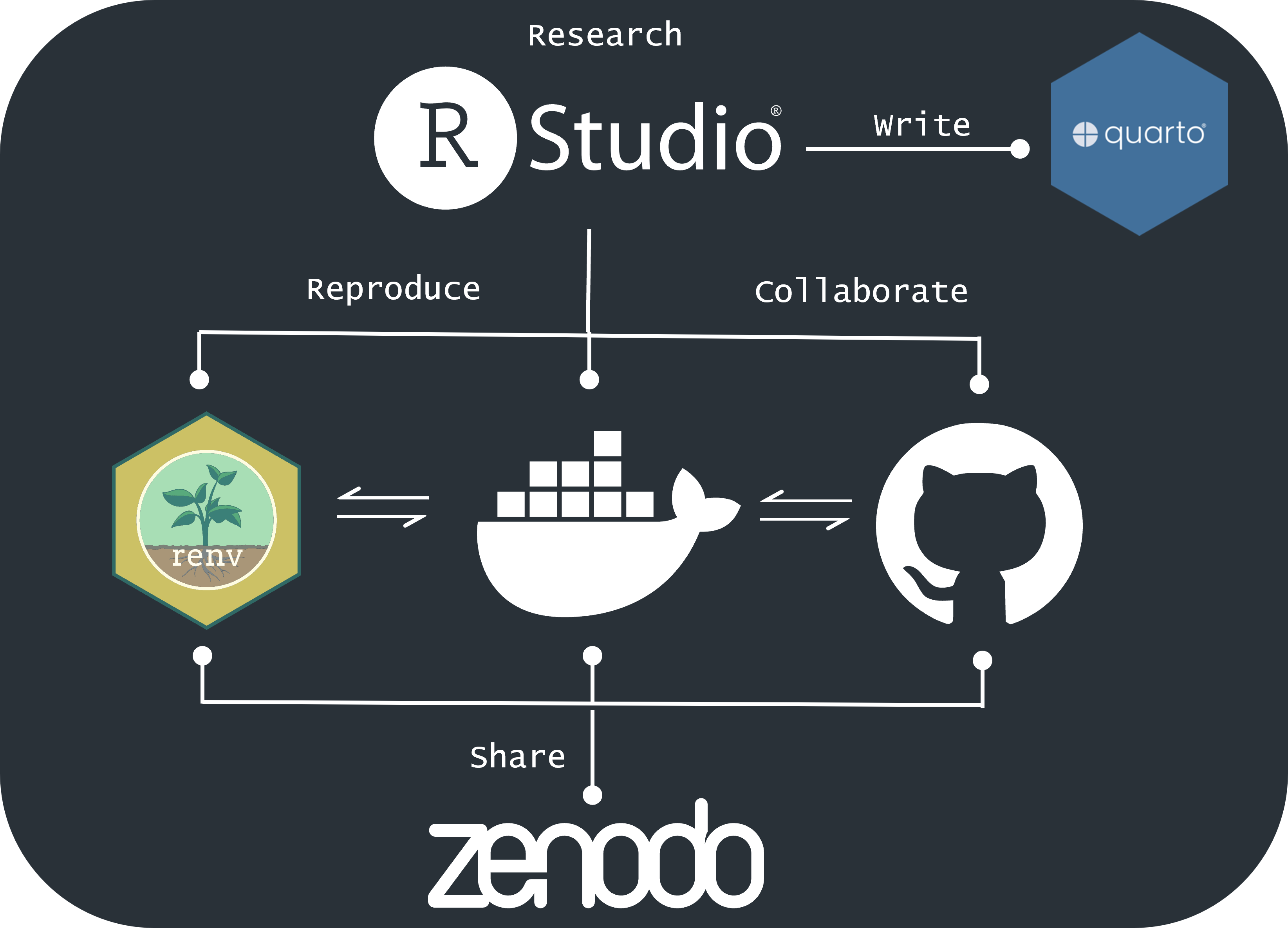


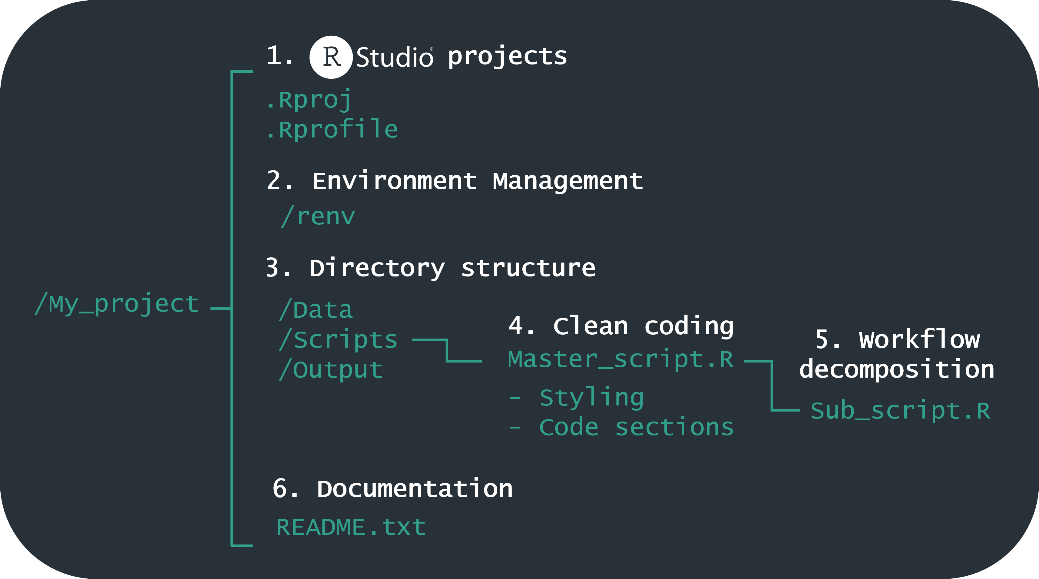
 projects
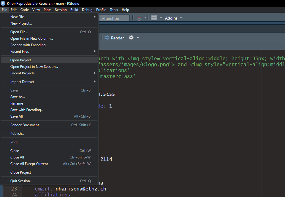
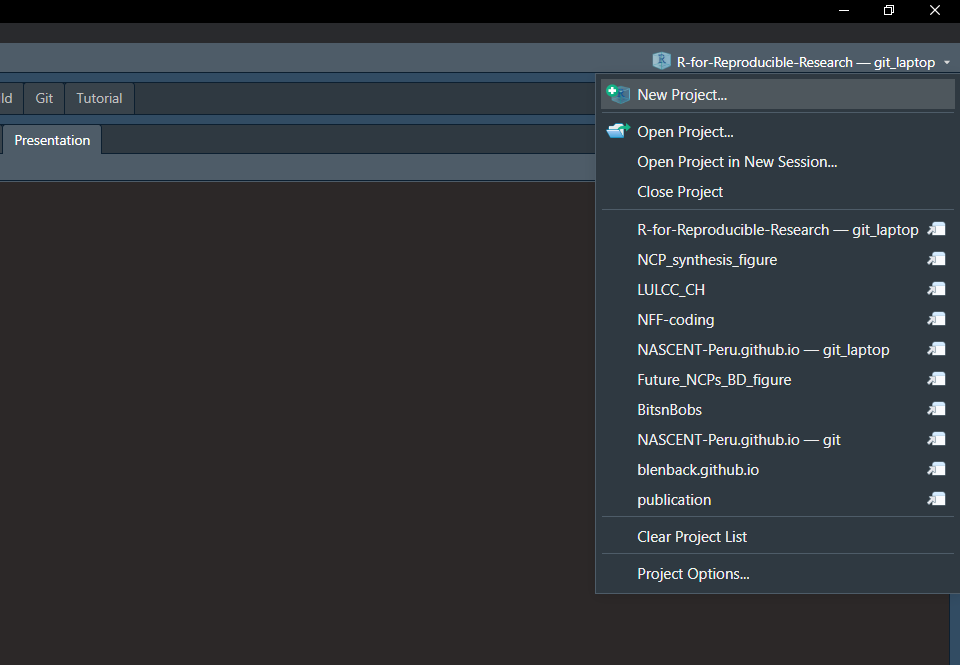
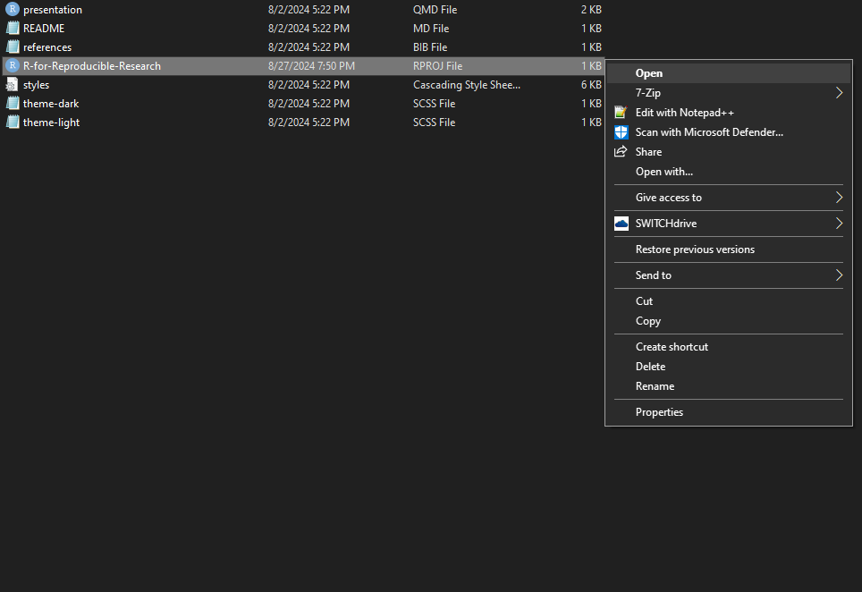
![Package dependencies of popular R package [13]](assets/images/package_dependencies_2.png)
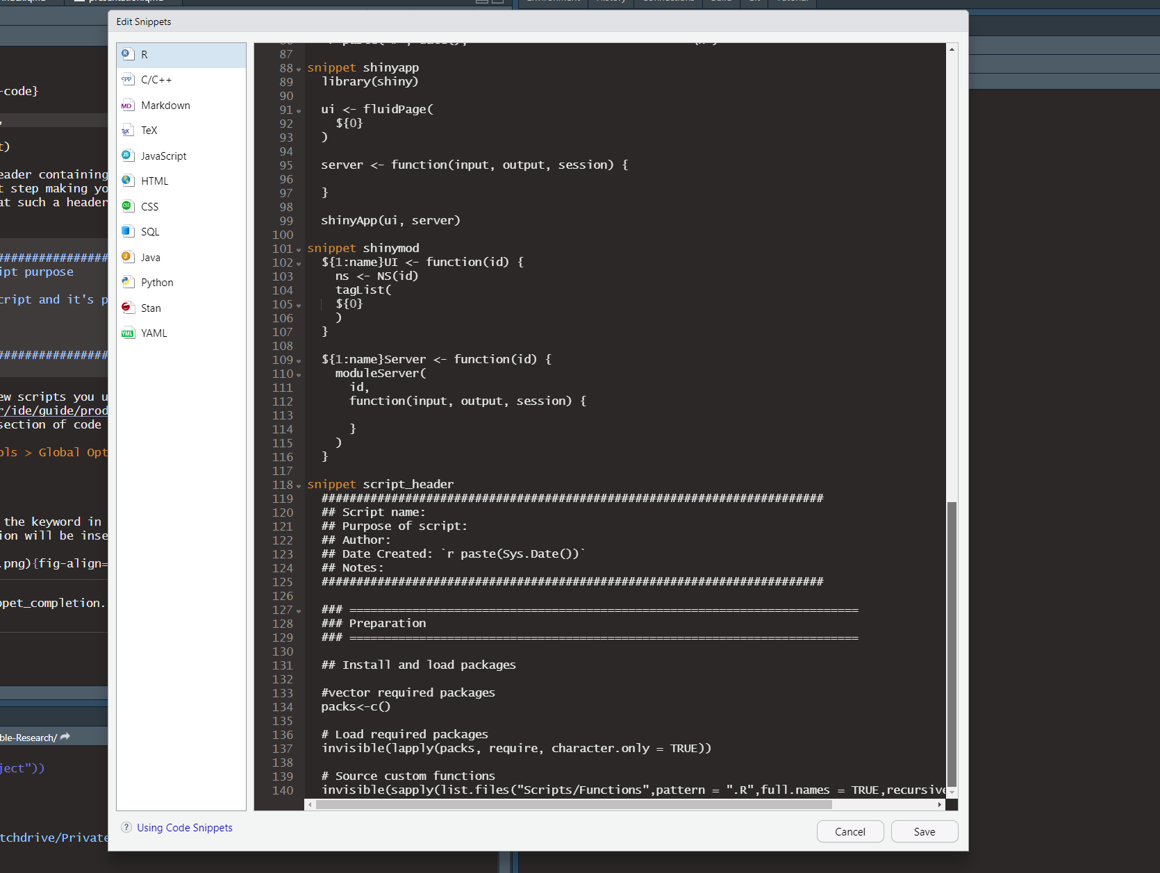
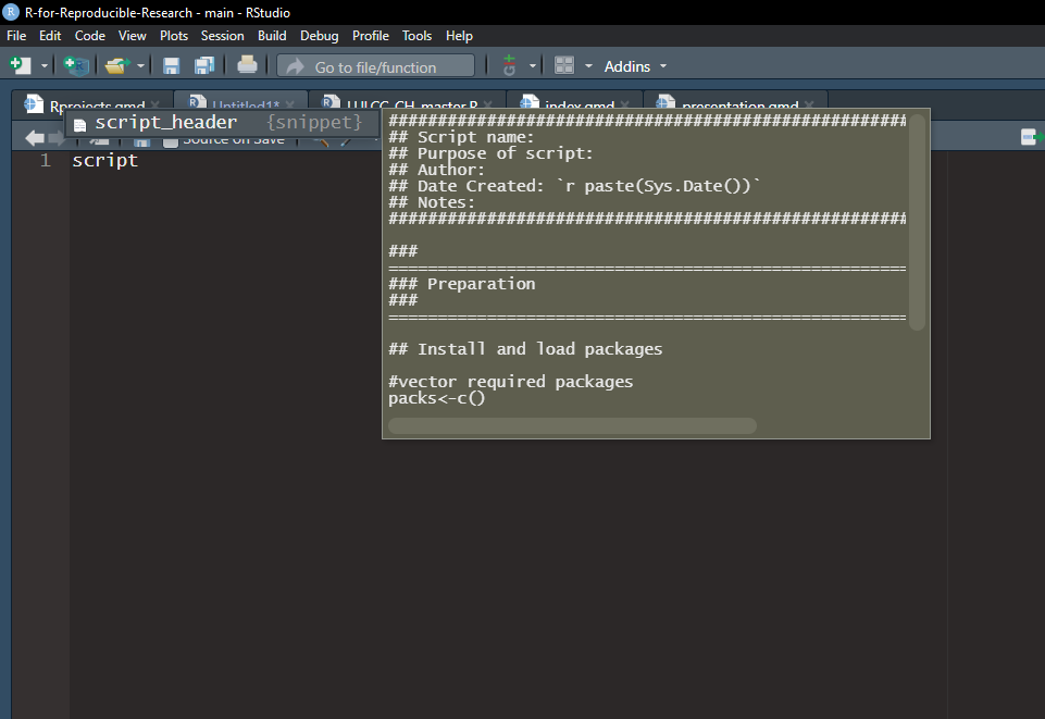


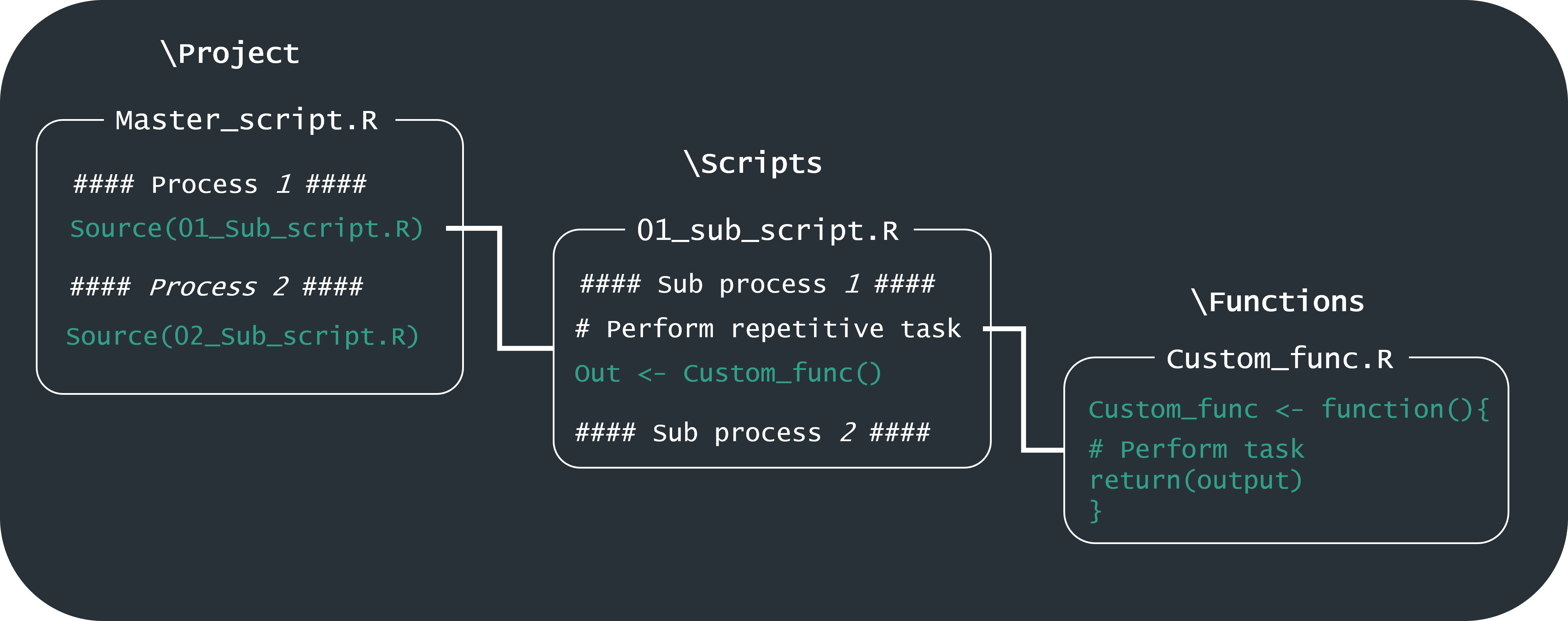
 pipeline

 project to
  pipeline
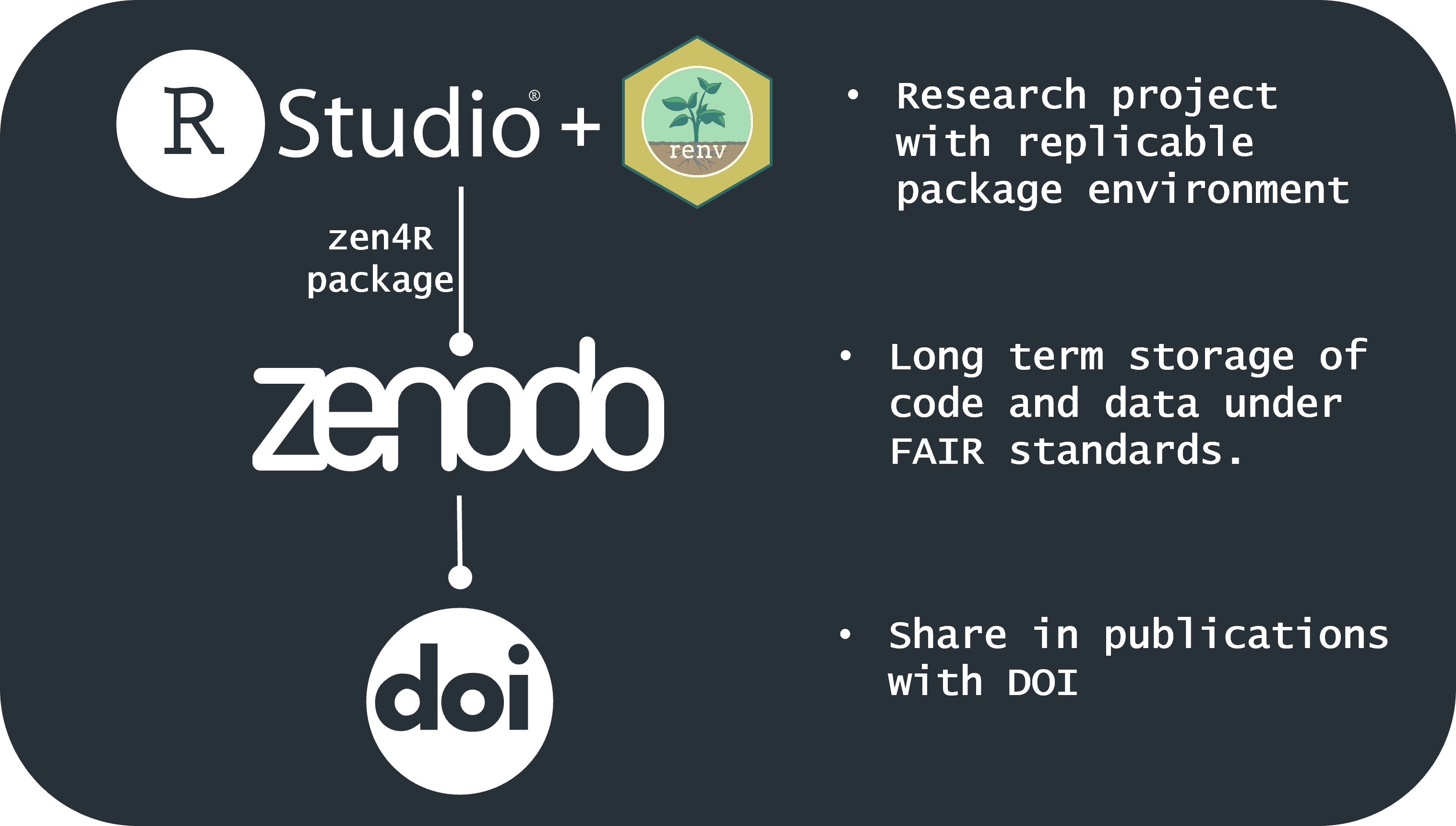
 as a research repository


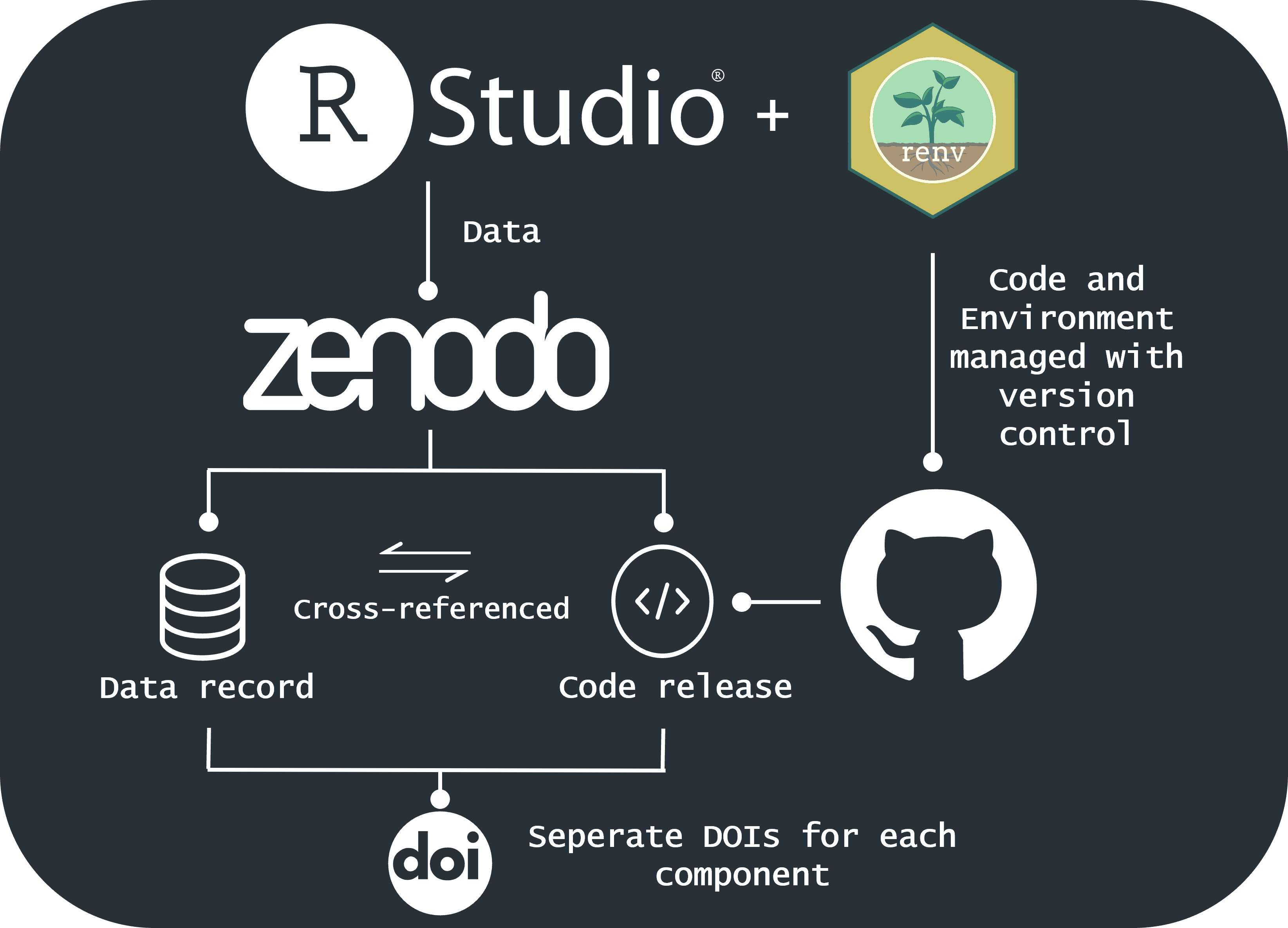
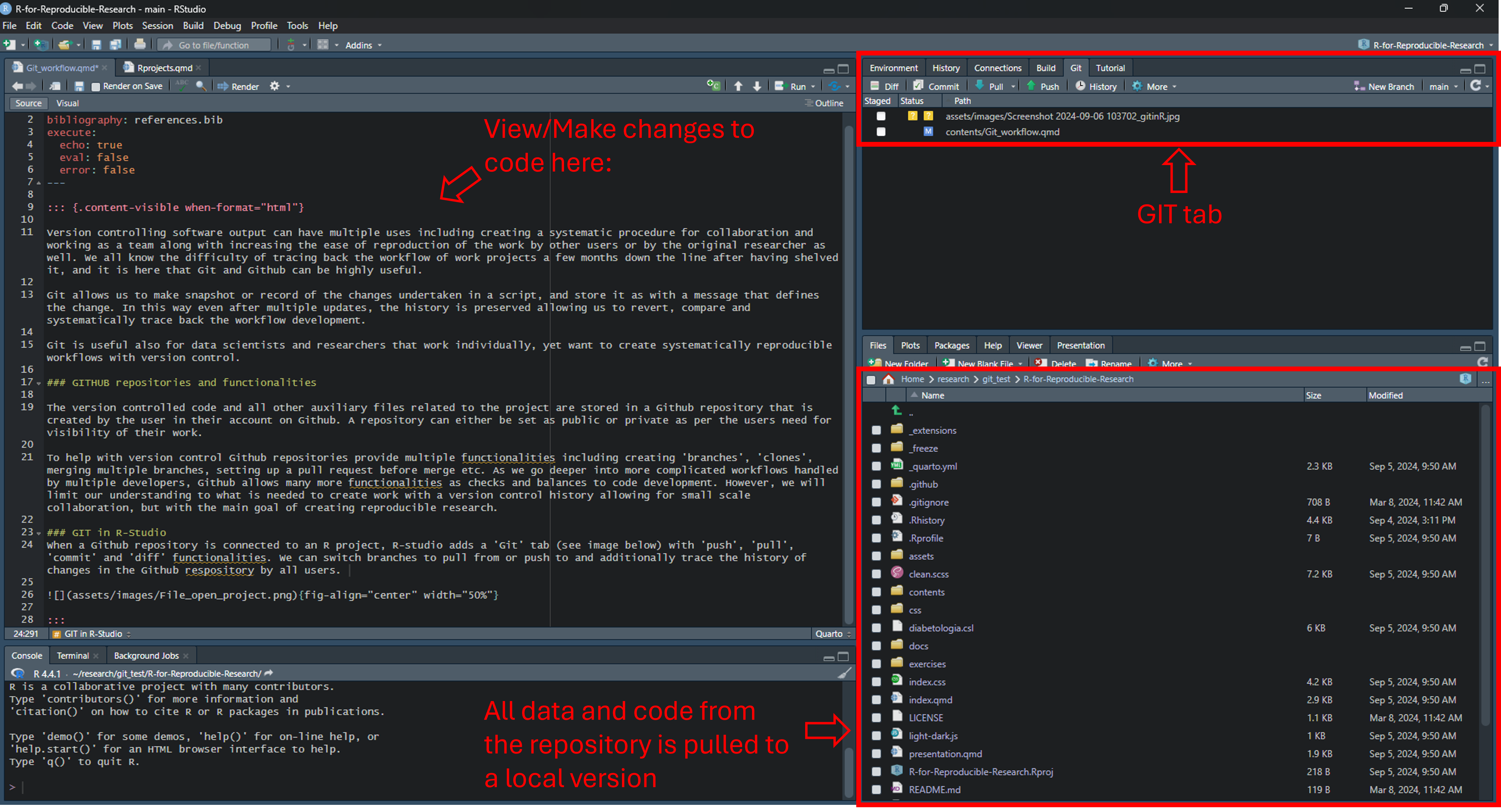
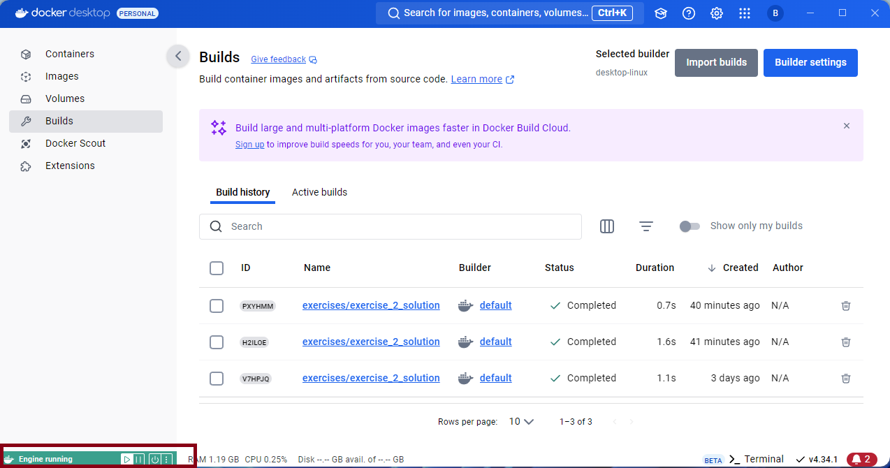
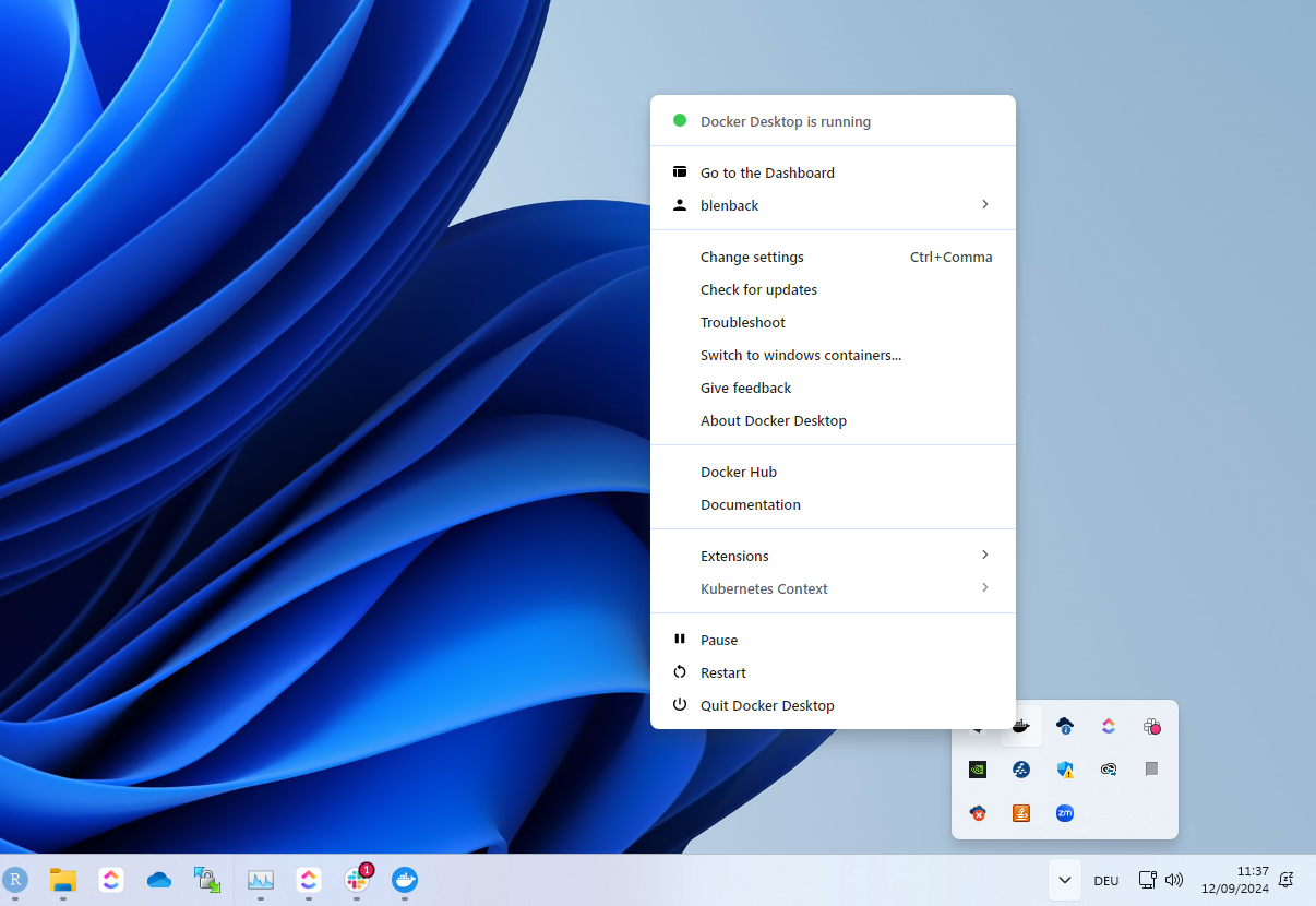
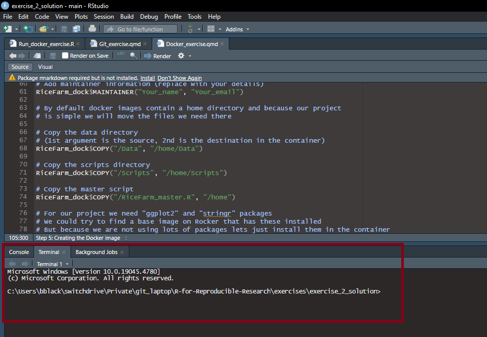
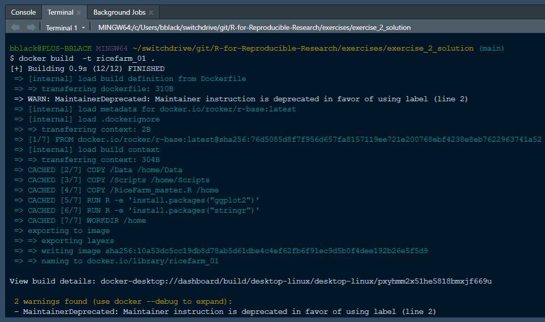
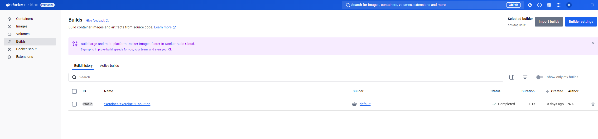
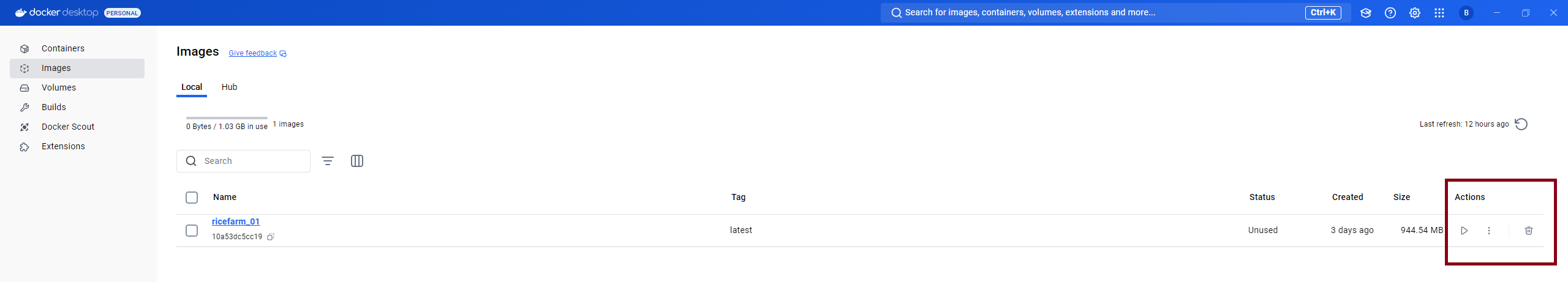
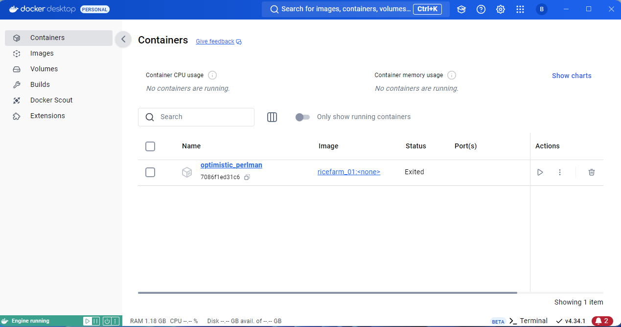
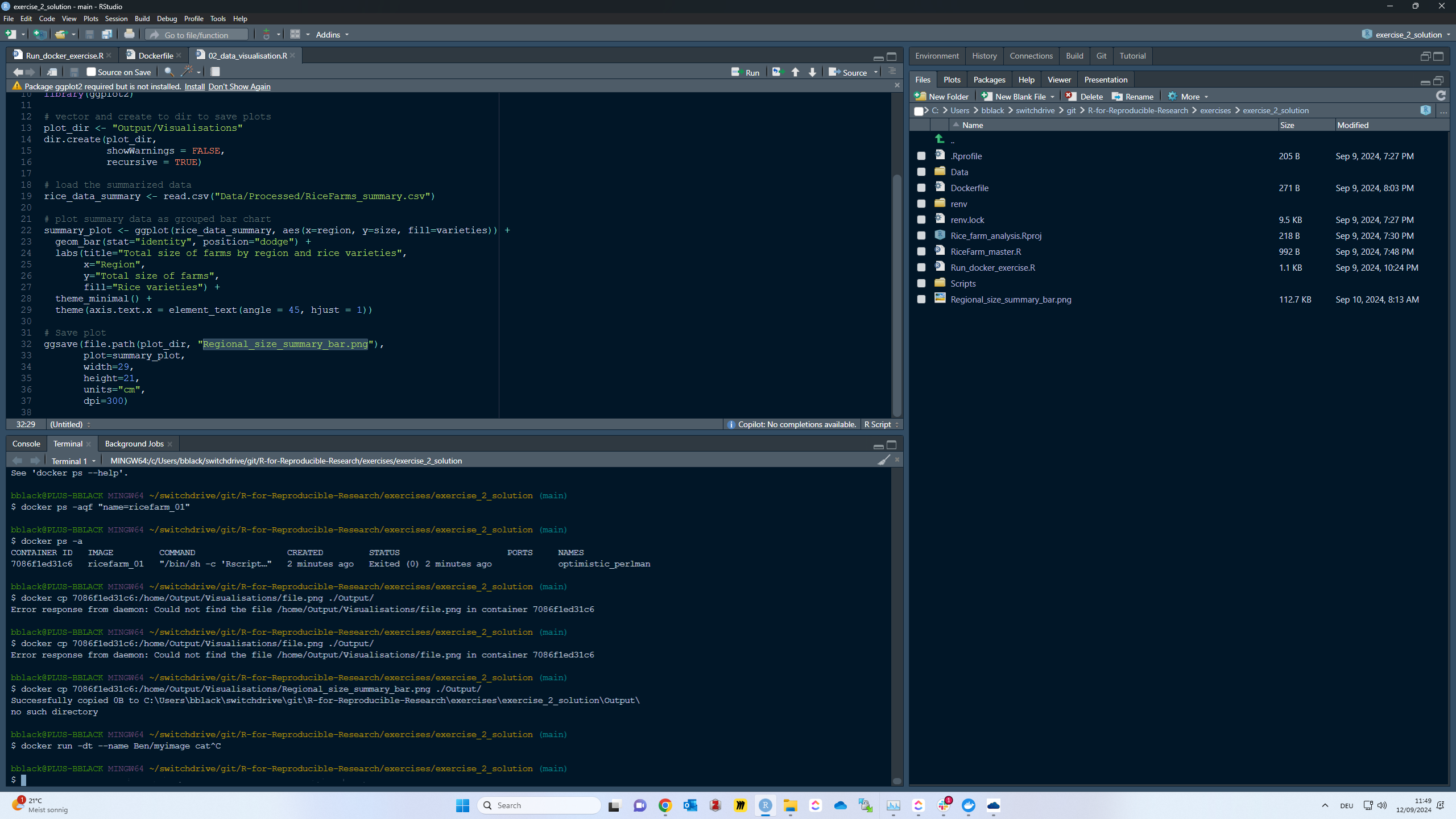

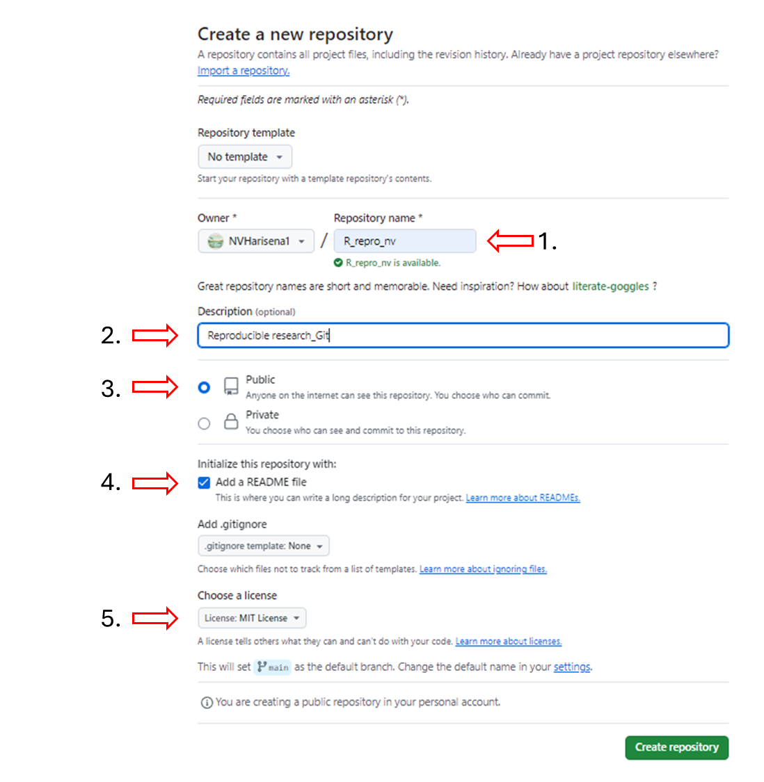
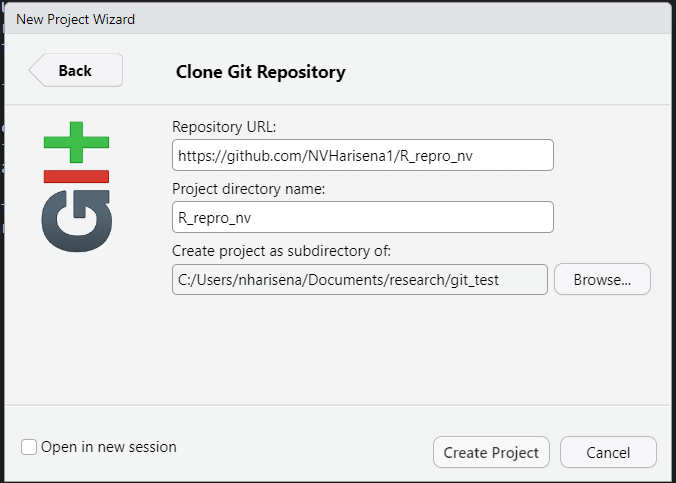
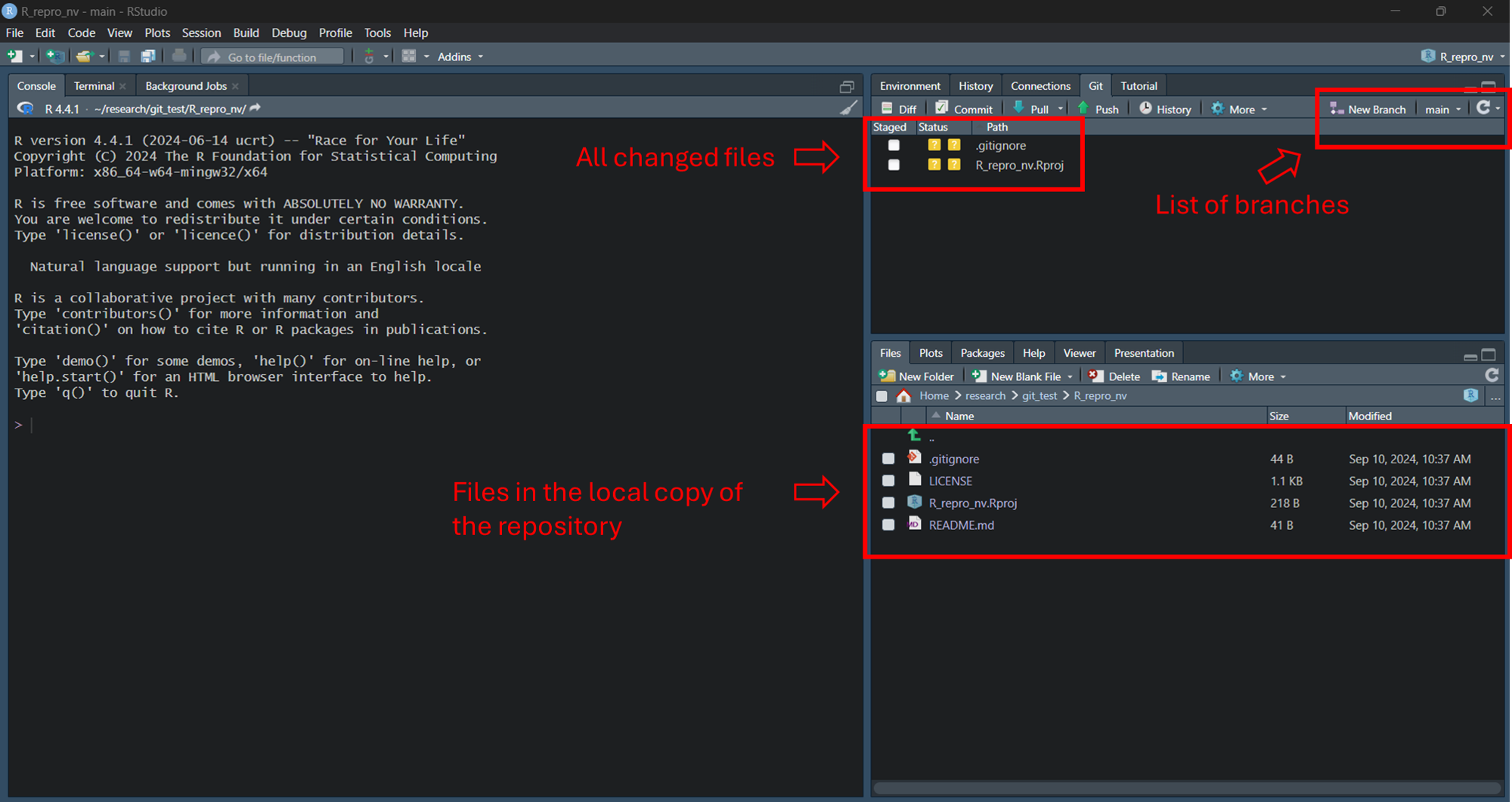
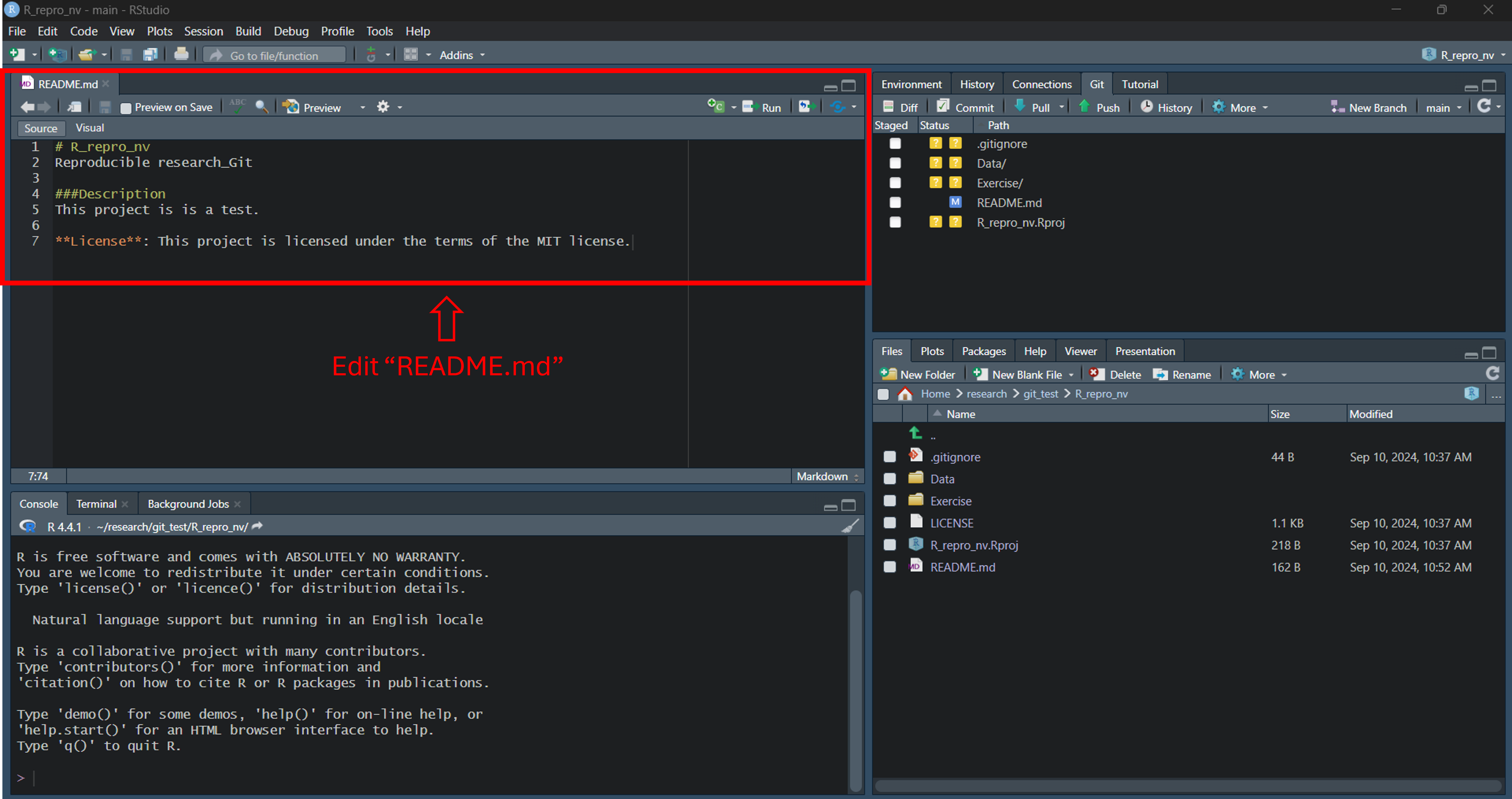
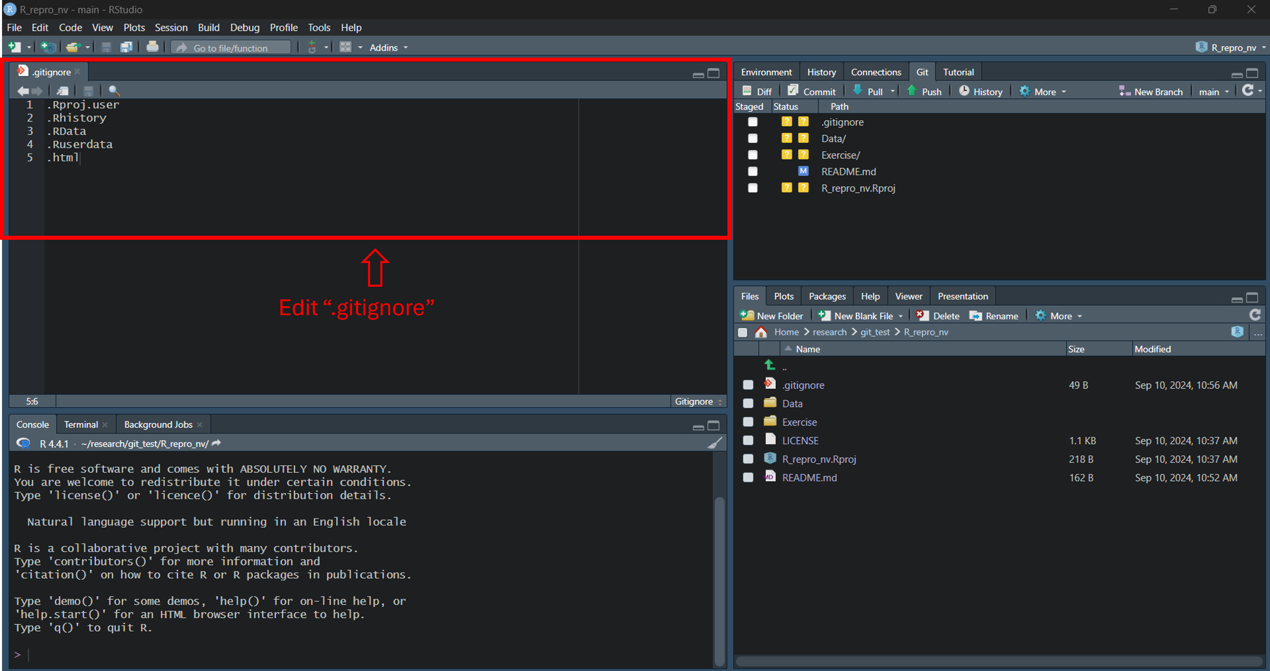
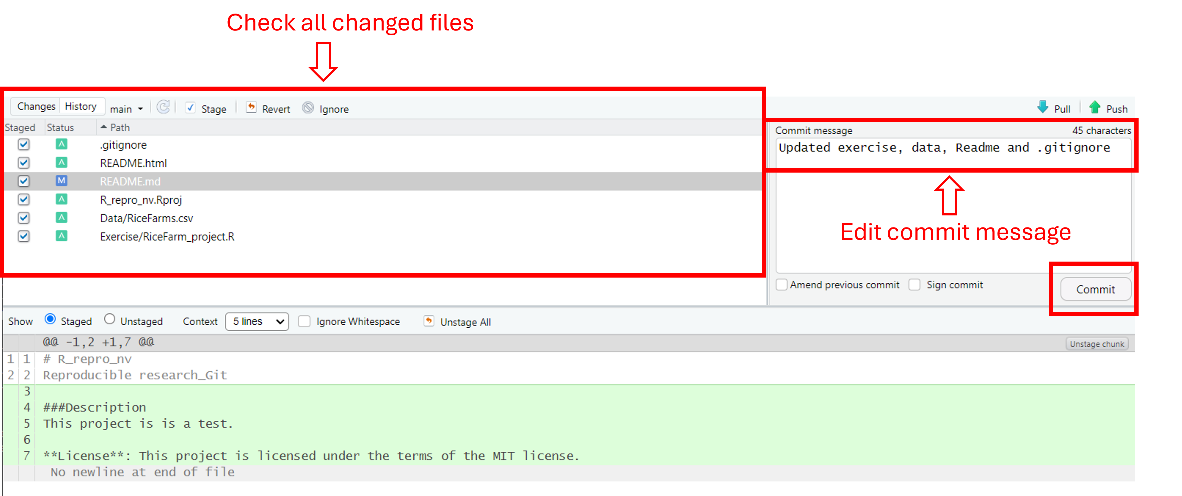
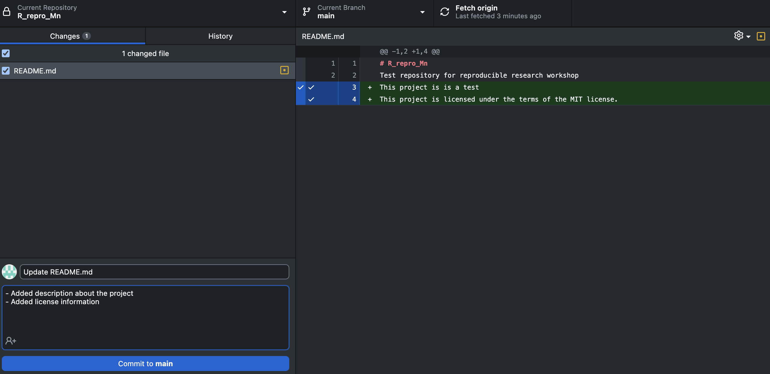
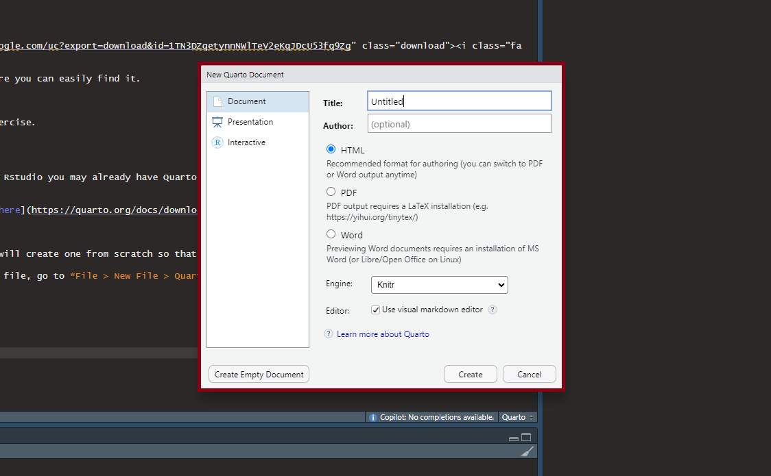
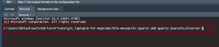
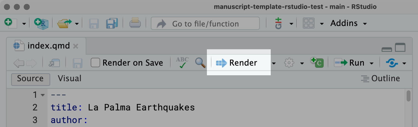
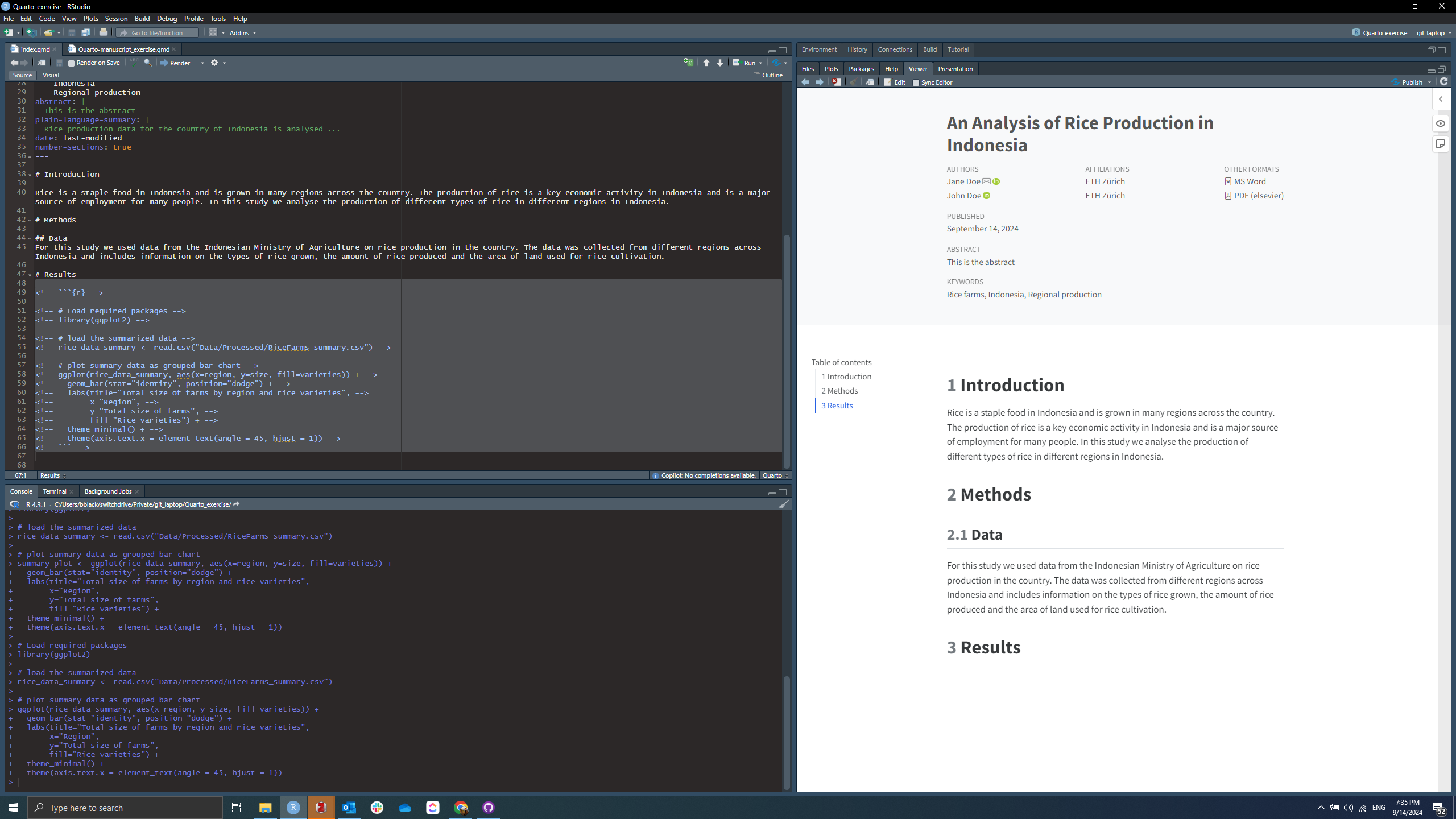
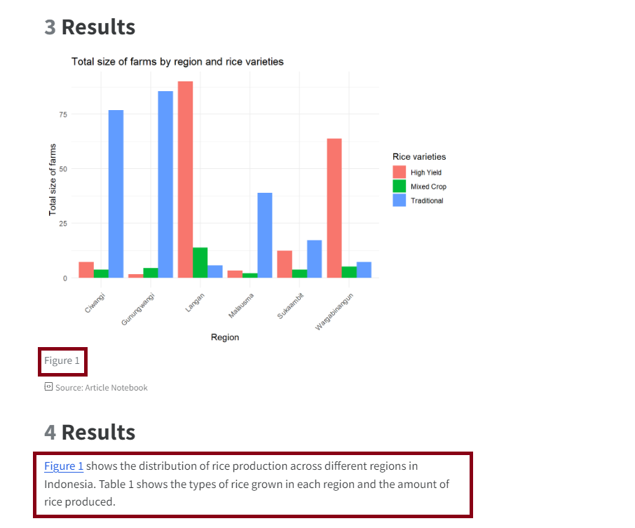
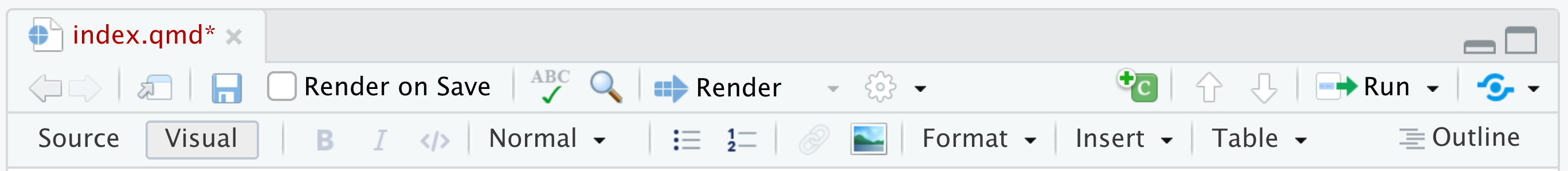
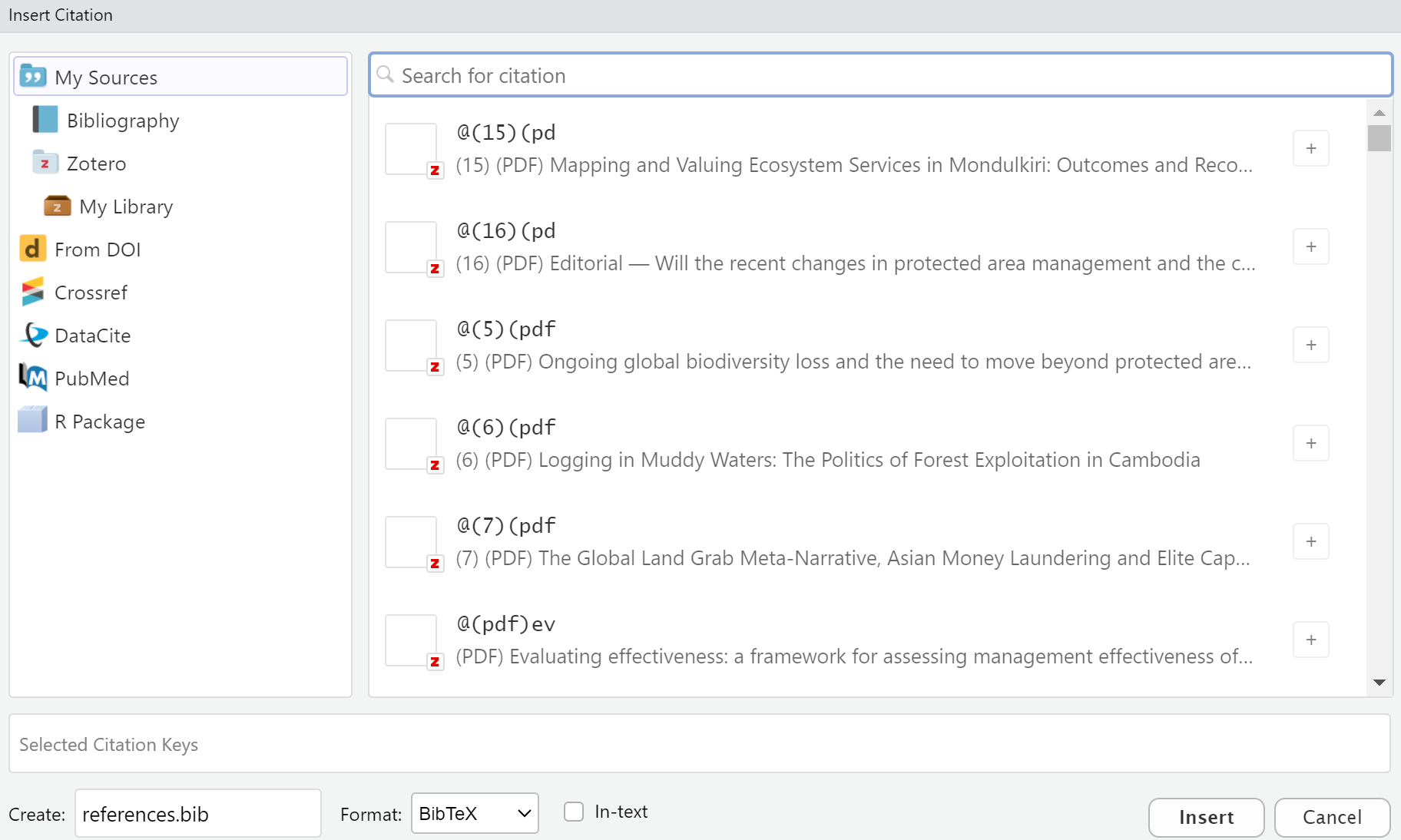
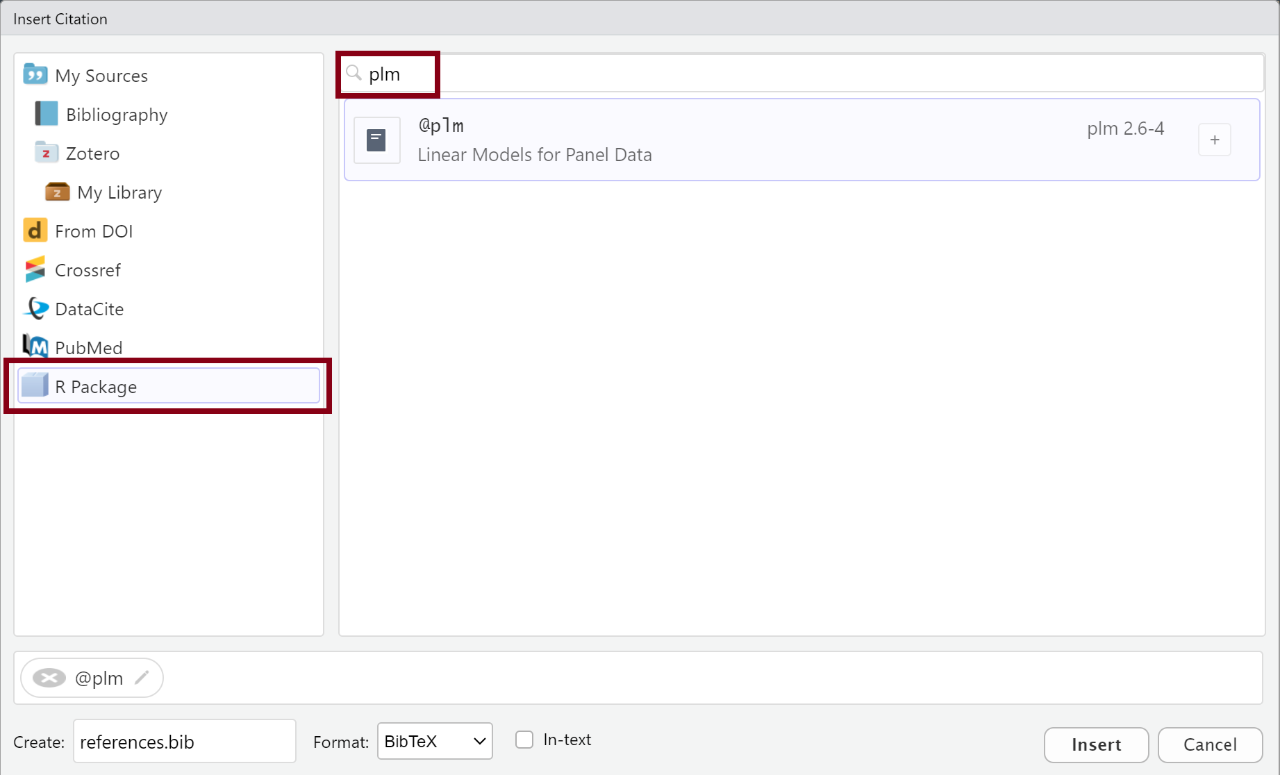
 to
to  to
to  pipeline] https://youtu.be/w3X76e_tZr8?si=bE4OfrNm-wLaeBlk